How to Grid Radar Data from Polar Sweeps to a Raster in Python

Problem statement

A radar sweep is a set of rays fanning out from the radar, each divided into range gates — a polar grid whose cells are 250 m long and get wider the further they are from the radar. To overlay it on a map, combine it with gauges or another radar, or save it as a GeoTIFF, it has to go onto a regular Cartesian grid. The two obvious ways to do that each fail somewhere: nearest-neighbour leaves holes far from the radar and throws away data near it, and averaging decibels gives the wrong answer everywhere.

This page grids the lowest sweep of the KHGX (Houston) radar during Hurricane Beryl's landfall on 8 July 2024 onto 1 km and 2 km grids, measures what each choice does, and writes a georeferenced GeoTIFF.

Quick answer

Bin every gate into the grid cell its centre falls in and average in linear reflectivity units, not decibels; choose a cell size the outer range can fill:

def grid_sweep(sw, res, half_width=250_000):
    n = int(2 * half_width / res)
    x, y, dbz = sw.x.values.ravel(), sw.y.values.ravel(), sw.DBZH.values.ravel()
    dbz = np.where(dbz > -32, dbz, np.nan)                 # -33 dBZ is the "below threshold" code, not an echo
    inside = (np.abs(x) < half_width) & (np.abs(y) < half_width)
    cell = ((half_width - y[inside]) // res).astype(int) * n + ((x[inside] + half_width) // res).astype(int)
    gates = np.bincount(cell, minlength=n * n)
    echo = np.isfinite(dbz[inside])
    z_lin = np.bincount(cell[echo], weights=10 ** (dbz[inside][echo] / 10), minlength=n * n)
    hits = np.bincount(cell[echo], minlength=n * n)
    with np.errstate(divide="ignore", invalid="ignore"):
        out = np.where(hits > 0, 10 * np.log10(z_lin / hits), np.nan)
    return out.reshape(n, n), gates.reshape(n, n)

g2, gates2 = grid_sweep(sweep, 2000)
print(g2.shape, f"cells with echo {np.isfinite(g2).sum():,}; max {np.nanmax(g2):.1f} dBZ")

(250, 250) cells with echo 24,959; max 51.4 dBZ

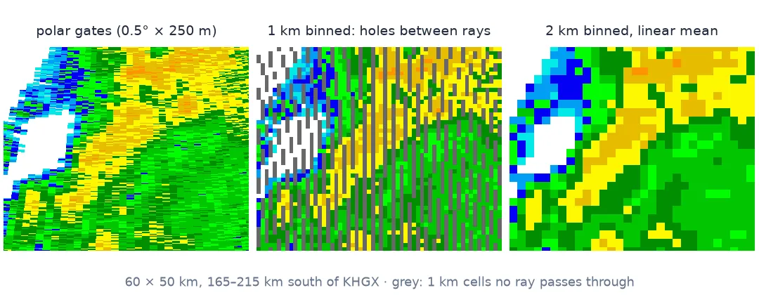
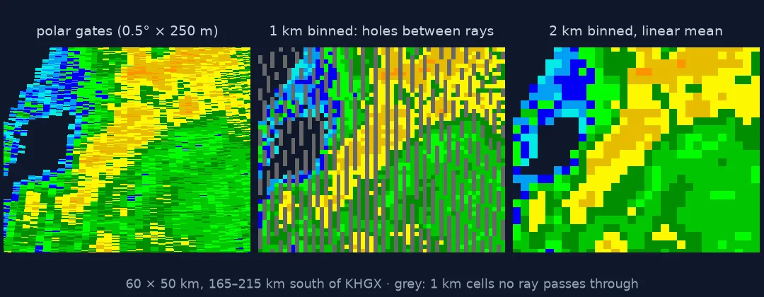
Polar cell sizes, the no-echo code, gates per cell

1. Know how big the polar cells are

Every gate is 250 m long, but its width is the range times the beam's angular spacing — half a degree on KHGX's low tilts:

for r_km in (20, 100, 200):
    print(f"{r_km:3d} km: gate {250} m long, {r_km * 1000 * np.radians(0.5):5.0f} m wide")

 20 km: gate 250 m long,   175 m wide
100 km: gate 250 m long,   873 m wide
200 km: gate 250 m long,  1745 m wide

Near the radar dozens of gates fall in each kilometre cell; at 200 km a ray is wider than a kilometre, and some 1 km cells fall between rays altogether.

2. Drop the "no echo" code

Every gate in the file has a value. Gates with no detectable echo carry the minimum, −33 dBZ, rather than a missing value:

raw = sweep.DBZH.values
print(f"gates: {raw.size:,}; at -33 dBZ (below threshold): {(raw <= -32).mean():.0%}; missing: {np.isnan(raw).mean():.0%}")

gates: 1,319,040; at -33 dBZ (below threshold): 63%; missing: 0%

Left in, they enter every average as a real, very weak echo and drag cells at the edge of the rain down. grid_sweep sets them to NaN first.

3. Count gates per cell before choosing a resolution

for res in (1000, 2000):
    g, gates = grid_sweep(sweep, res)
    n = g.shape[0]
    centre = (np.arange(n) + 0.5) * res - 250_000
    rr = np.hypot(*np.meshgrid(centre, -centre))
    holes = (gates == 0) & (rr < 240_000)
    print(f"{res / 1000:.0f} km grid: gates per cell at 20 / 100 / 200 km: "
          f"{gates[np.abs(rr - 20e3) < res].mean():.0f} / {gates[np.abs(rr - 100e3) < res].mean():.1f} / "
          f"{gates[np.abs(rr - 200e3) < res].mean():.1f}; cells with no gate inside 240 km: {holes.sum():,}")

1 km grid: gates per cell at 20 / 100 / 200 km: 23 / 4.5 / 2.3; cells with no gate inside 240 km: 34,094
2 km grid: gates per cell at 20 / 100 / 200 km: 92 / 18.3 / 9.1; cells with no gate inside 240 km: 3

A 1 km grid leaves cells with no gate at all at long range; at 2 km every cell inside 240 km gets several. Choose the resolution the far range supports, or interpolate across the holes deliberately.

4. Average in linear units

Reflectivity in dBZ is logarithmic. The average of 20 dBZ and 40 dBZ is not 30 dBZ: in linear units (mm⁶/m³) it is 100 and 10,000, averaging to 5,050, which is 37 dBZ. Averaging decibels systematically underestimates:

x, y, dbz = (sweep[v].values.ravel() for v in ("x", "y", "DBZH"))
ok = (dbz > -32) & (np.abs(x) < 250_000) & (np.abs(y) < 250_000)
cell = ((250_000 - y[ok]) // 2000).astype(int) * 250 + ((x[ok] + 250_000) // 2000).astype(int)
cnt = np.bincount(cell, minlength=250 * 250)
with np.errstate(divide="ignore"):
    lin = 10 * np.log10(np.bincount(cell, weights=10 ** (dbz[ok] / 10), minlength=250 * 250) / np.maximum(cnt, 1))
db = np.bincount(cell, weights=dbz[ok], minlength=250 * 250) / np.maximum(cnt, 1)
m = (cnt > 0) & (lin > 20)
print(f"linear mean minus dB mean, cells above 20 dBZ: average {np.mean((lin - db)[m]):.2f} dB, 95th percentile {np.percentile((lin - db)[m], 95):.1f} dB")

linear mean minus dB mean, cells above 20 dBZ: average 0.90 dB, 95th percentile 1.9 dB

About a decibel on average and up to two in the cells with the most variable echo — and since rain rate depends steeply on reflectivity, a decibel matters.

5. Write a GeoTIFF

The grid is in the radar's azimuthal equidistant projection, centred on the radar. Write it with that CRS and let GIS software reproject:

aeqd = CRS.from_proj4(f"+proj=aeqd +lat_0={float(dt.ds.latitude)} +lon_0={float(dt.ds.longitude)} +units=m +datum=WGS84")
transform = from_origin(-250_000, 250_000, 2000, 2000)
with rasterio.open("data/khgx_20240708_0901_dbz_2km.tif", "w", driver="GTiff", height=g2.shape[0], width=g2.shape[1],
                   count=1, dtype="float32", crs=aeqd, transform=transform, nodata=np.nan, compress="deflate") as dst:
    dst.write(g2.astype("float32"), 1)
with rasterio.open("data/khgx_20240708_0901_dbz_2km.tif") as src:
    print(src.crs.to_proj4(), src.res, [round(v) for v in transform_bounds(src.crs, 4326, *src.bounds)])

+proj=aeqd +lat_0=29.4719009399414 +lon_0=-95.0787353515625 +x_0=0 +y_0=0 +datum=WGS84 +units=m +no_defs=True (2000.0, 2000.0) [-98, 27, -92, 32]

Nearest-neighbour and latitude-longitude grids

The data used on this page

NOAA NEXRAD Level II, KHGX (Houston/Galveston), volume 2024-07-08 09:01:25 UTC, from the Unidata NEXRAD Level II archive on AWS.

from pathlib import Path

import numpy as np
import rasterio
import requests
import xradar as xd
from pyproj import CRS
from rasterio.transform import from_origin
from rasterio.warp import transform_bounds

Path("data").mkdir(exist_ok=True)
KEY = "2024/07/08/KHGX/KHGX20240708_090125_V06"
path = Path("data") / KEY.split("/")[-1]
if not path.exists():
    path.write_bytes(requests.get("https://unidata-nexrad-level2.s3.amazonaws.com/" + KEY, timeout=300).content)
dt = xd.io.open_nexradlevel2_datatree(str(path)).xradar.georeference()
sweep = dt["sweep_0"].ds
print(sweep.DBZH.shape, float(sweep.sweep_fixed_angle))

(720, 1832) 0.4833984375

Example 1: nearest-neighbour for comparison

Nearest-neighbour takes one gate per cell and discards the rest:

from scipy.spatial import cKDTree
pts = np.c_[x[ok], y[ok]]
tree = cKDTree(pts)
centre = (np.arange(250) + 0.5) * 2000 - 250_000
GX, GY = np.meshgrid(centre, -centre)
d, i = tree.query(np.c_[GX.ravel(), GY.ravel()])
nn = np.where(d < 2000, dbz[ok][i], np.nan).reshape(250, 250)
both = np.isfinite(nn) & np.isfinite(g2)
print(f"nearest minus binned linear mean: median {np.median((nn - g2)[both]):+.2f} dB, "
      f"5th-95th {np.percentile((nn - g2)[both], 5):+.1f} to {np.percentile((nn - g2)[both], 95):+.1f} dB")

nearest minus binned linear mean: median -0.71 dB, 5th-95th -5.7 to +3.1 dB

Nearest-neighbour lets one gate stand in for dozens. It reads 0.7 dB below the linear mean in the median — a single gate's value, like a decibel average, sits below the mean power — and scatters by several decibels either way, so the grid inherits each chosen gate's speckle.

Example 2: put it on a latitude–longitude map

from rasterio.warp import calculate_default_transform, reproject, Resampling
with rasterio.open("data/khgx_20240708_0901_dbz_2km.tif") as src:
    t, w, h = calculate_default_transform(src.crs, "EPSG:4326", src.width, src.height, *src.bounds)
    ll = np.full((h, w), np.nan, np.float32)
    reproject(src.read(1), ll, src_transform=src.transform, src_crs=src.crs, dst_transform=t, dst_crs="EPSG:4326",
              resampling=Resampling.nearest)
print(ll.shape, f"{t.a:.4f} deg pixels")

(234, 272) 0.0194 deg pixels

A change of sampling from polar to Cartesian

Gridding radar data is a change of sampling, from a polar grid that is dense near the radar and sparse far away to a Cartesian grid that is the same everywhere. No single method handles both ends. Near the radar there are far more gates than cells, so the question is how to combine them; far away there are fewer, so the question is how to fill cells that no gate reaches.

Binning with a linear average answers the first: every gate contributes, and averaging in Z rather than dBZ respects that reflectivity is a power, not a level. Choosing a cell size that the outermost range can still fill answers the second without inventing values; finer grids at long range need explicit interpolation and should say so. Libraries such as Py-ART and wradlib offer gridding with radius-of-influence interpolation for exactly this, and the same two decisions — average in which units, fill which gaps — sit inside them.

Linear averaging and no echo against zero

• Average in linear units (10^(dBZ/10)), then convert back.
• Cell size vs gate width: at 200 km a 0.5° ray is 1.7 km wide.
• −33 dBZ means no echo: mask it before averaging.
• No echo is not zero: keep cells with gates but no echo separate from cells with no gates.
• Use the radar-centred projection for gridding; reproject after.
• Higher tilts cover shorter ground ranges; a composite needs all of them.
• Beam height grows with range; the grid is not at a single altitude.

Internal links

• How to read NEXRAD Level II — the sweep used here
• Weather radar reflectivity explained — why dBZ is logarithmic
• How to estimate rainfall from radar — the next step
• Radar beam blockage and clutter — gates to drop before gridding
• How to map storm-total rainfall — grids accumulated over time

FAQ

How do I convert radar polar data to a grid in Python?

Georeference the sweep to x and y, bin each gate into a Cartesian cell, and average in linear reflectivity units; write the result with an azimuthal equidistant CRS centred on the radar.

Should I average dBZ values?

No. Convert to linear Z, average, and convert back. Averaging dBZ underestimated by about 1 dB on average in this sweep.

What grid resolution should I use for radar data?

One that the outer range can fill: at 200 km a 0.5° beam is 1.7 km wide, so a 2 km grid has gates in every cell while a 1 km grid has holes.

What projection is radar data in?

Natively polar, centred on the radar; gridded products are usually written in an azimuthal equidistant projection centred on the radar.