
Radar Rainfall vs Rain Gauges Explained: Why They Disagree
On this page
Problem statement
Put a radar rainfall estimate next to the rain gauges under it and they disagree. Sometimes by a few percent, sometimes by a factor of two at one gauge and the opposite at its neighbour. It is tempting to call one of them truth and the other error. Neither is truth: they measure different things, at different places, over different times. Most of the disagreement can be traced to those differences before anything is wrong with either instrument.
This page takes the MRMS radar-only estimate for Hurricane Beryl's rain around Houston in July 2024 and the 80-odd volunteer and official gauges under it. It separates the disagreement into its parts: timing, distance from the radar, the scale mismatch between a gauge and a grid cell, and the gauges' own scatter.
Quick answer
Compare radar and gauges over the same window, at more than one scale, and look at how the ratio changes with distance from the radar:
for label, g in (("one day (CoCoRaHS dated 9 July)", DAY), ("storm total (7-10 July)", STORM)):
    print(f"{label}: n = {len(g)}, r = {np.corrcoef(g.gauge, g.radar)[0, 1]:.2f}, "
          f"median radar/gauge {(g.radar / g.gauge).median():.2f}")
    for lo, hi in ((0, 40), (40, 80), (80, 150)):
        m = g.km.between(lo, hi, inclusive="left")
        print(f"   {lo:3d}-{hi:3d} km from KHGX: {m.sum():2d} gauges, radar/gauge {g.radar[m].sum() / g.gauge[m].sum():.2f}")
one day (CoCoRaHS dated 9 July): n = 83, r = 0.75, median radar/gauge 0.95
0- 40 km from KHGX: 19 gauges, radar/gauge 1.38
40- 80 km from KHGX: 24 gauges, radar/gauge 0.98
80-150 km from KHGX: 40 gauges, radar/gauge 0.80
storm total (7-10 July): n = 75, r = 0.74, median radar/gauge 1.08
0- 40 km from KHGX: 19 gauges, radar/gauge 1.16
40- 80 km from KHGX: 25 gauges, radar/gauge 1.13
80-150 km from KHGX: 31 gauges, radar/gauge 1.05
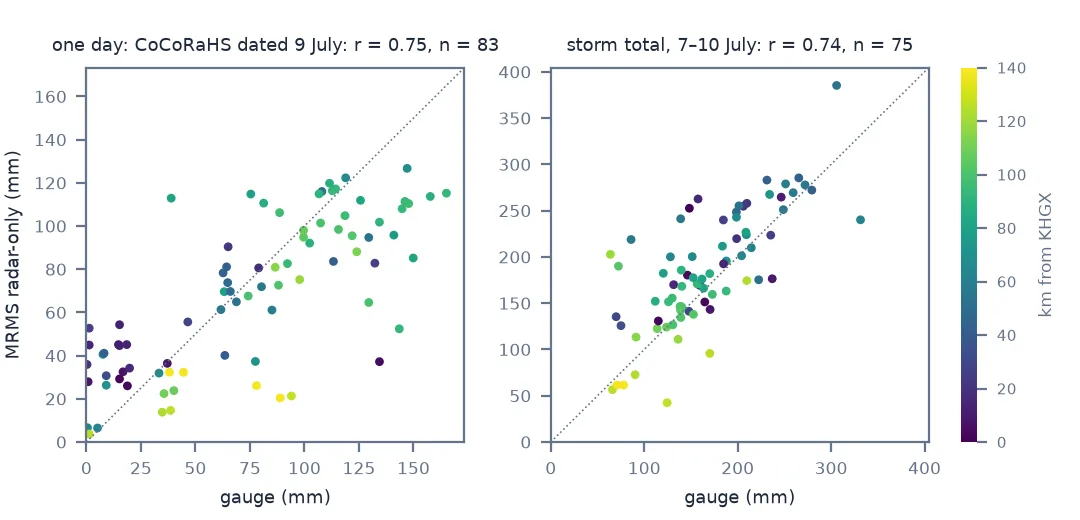
Different quantities, aligned windows, gauges that disagree
1. They measure different things
A gauge catches the rain falling into an opening about 20 cm across at the ground. A radar estimate is a reflectivity measured in a beam a kilometre or more deep. That beam sits hundreds of metres to kilometres up and is converted to rain by an assumed drop-size relationship. It is then mapped to a 1 km cell, about 30 million times the gauge's catchment area. Rain varies inside that cell:
spread = []
for la, lo in zip(STORM.LATITUDE, STORM.LONGITUDE):
    i = int(np.argmin(np.abs(RO_STORM.latitude.values - la)))
    j = int(np.argmin(np.abs(RO_STORM.longitude.values - lo % 360)))
    w = RO_STORM.values[i - 1:i + 2, j - 1:j + 2]
    spread.append(np.nanmax(w) - np.nanmin(w))
print(f"3 x 3 km around each gauge, radar storm totals vary by a median {np.median(spread):.1f} mm "
      f"({np.median(np.array(spread) / STORM.radar):.0%} of the cell value)")
3 x 3 km around each gauge, radar storm totals vary by a median 23.9 mm (15% of the cell value)
2. Line up the time windows
Most CoCoRaHS observers read their gauge at about 7 am and date the reading that morning, but not all. The radar estimate here is a 24-hour accumulation ending 12 UTC (7 am in Houston), so it matches only those who read on time:
low = DAY[DAY.gauge < 0.5 * DAY.radar]
print(f"{len(low)} of {len(DAY)} gauges caught less than half the radar estimate on 9 July; "
      f"{(low.km < 40).sum()} of them within 40 km of KHGX")
same = STORM[STORM.STATION.isin(low.STATION)]
print(f"{len(same)} of them reported every day of the storm; their storm totals: median radar/gauge "
      f"{(same.radar / same.gauge).median():.2f}")
15 of 83 gauges caught less than half the radar estimate on 9 July; 9 of them within 40 km of KHGX
9 of them reported every day of the storm; their storm totals: median radar/gauge 1.07
Of those 15, the 9 that reported every day of the storm agree with the radar once the whole storm is summed (median ratio 1.07). They had logged part of the rain on 8 July. The near-radar bias in the quick answer shrinks from 1.38 to 1.16 for the same reason.
3. Gauges disagree with each other too
If two gauges a couple of kilometres apart differ, a radar cell cannot match both. Compare close pairs:
xy = np.c_[Transformer.from_crs(4326, 32615, always_xy=True).transform(STORM.LONGITUDE.values, STORM.LATITUDE.values)]
pairs = np.array(sorted(cKDTree(xy).query_pairs(3000)))
g_diff = np.abs(STORM.gauge.values[pairs[:, 0]] - STORM.gauge.values[pairs[:, 1]])
r_diff = np.abs(STORM.radar.values[pairs[:, 0]] - STORM.radar.values[pairs[:, 1]])
mean = STORM.gauge.values[pairs].mean(axis=1)
print(f"{len(pairs)} gauge pairs within 3 km: they differ by a median {np.median(g_diff):.1f} mm "
      f"({np.median(g_diff / mean):.0%}); the radar at the same pairs by {np.median(r_diff):.1f} mm")
11 gauge pairs within 3 km: they differ by a median 14.0 mm (9%); the radar at the same pairs by 8.7 mm
Neighbouring gauges disagree with each other more than the radar field varies across the same distance. Some of that is real small-scale variation; some is gauge error — siting, wind, and a volunteer's reading.
4. Look at distance from the radar
The remaining radar-only bias falls with distance from KHGX, from 1.16 within 40 km to 1.05 beyond 80 km. Close to the radar the beam is low enough to catch clutter. Farther out it is higher and wider, and on the single day the ratio fell to 0.80 beyond 80 km. Both effects depend on range, so a radar-gauge ratio should always be examined against it.
5. Do not validate against the gauges you calibrated with
MRMS's multi-sensor product is adjusted to gauges every hour. Comparing it with the same gauges measures the adjustment, not the radar:
for name, field in (("radar-only", "radar"), ("multi-sensor (gauge-adjusted)", "ms")):
    print(f"{name:30s}: r = {np.corrcoef(STORM.gauge, STORM[field])[0, 1]:.2f}, median ratio {(STORM[field] / STORM.gauge).median():.2f}")
radar-only : r = 0.74, median ratio 1.08
multi-sensor (gauge-adjusted) : r = 0.76, median ratio 0.96
How much each step explains
The data used on this page
MRMS RadarOnly and MultiSensor Pass 2 QPE from the NOAA MRMS archive on AWS: 24 h ending 12 UTC 9 July for the single day, and 24 h ending 12 UTC 7 July plus 72 h ending 12 UTC 10 July for the storm; GHCN-Daily precipitation for 7–10 July 2024 from the NCEI daily-summaries service. KHGX is at 29.4719° N, 95.0787° W.
import gzip
import shutil
from pathlib import Path

import numpy as np
import pandas as pd
import requests
import xarray as xr
from pyproj import Geod, Transformer
from scipy.spatial import cKDTree

Path("data").mkdir(exist_ok=True)


def fetch(url, name):
    if not Path("data", name).exists():
        Path("data", name).write_bytes(requests.get(url, timeout=600).content)
    return Path("data", name)


def mrms(product, stamp):
    name = f"MRMS_{product}_00.00_{stamp}.grib2"
    gz = fetch(f"https://noaa-mrms-pds.s3.amazonaws.com/CONUS/{product}_00.00/{stamp[:8]}/{name}.gz", name + ".gz")
    if not Path("data", name).exists():
        with gzip.open(gz) as src, open(Path("data", name), "wb") as dst:
            shutil.copyfileobj(src, dst)
    q = xr.open_dataset(Path("data", name), engine="cfgrib", decode_timedelta=True, backend_kwargs={"indexpath": ""})["unknown"]
    return q.where(q >= 0)


inv = pd.read_fwf(fetch("https://www.ncei.noaa.gov/pub/data/ghcn/daily/ghcnd-inventory.txt", "ghcnd-inventory.txt"),
                  widths=[11, 9, 10, 5, 5, 5], names=["id", "lat", "lon", "el", "first", "last"])
ids = inv[(inv.el == "PRCP") & (inv["last"] >= 2024) & inv.lat.between(28.8, 30.4) & inv.lon.between(-96.3, -94.6)].id.unique()
if not Path("data/gauges.csv").exists():
    parts = []
    for i in range(0, len(ids), 90):
        text = requests.get("https://www.ncei.noaa.gov/access/services/data/v1", timeout=300, params={
            "dataset": "daily-summaries", "dataTypes": "PRCP", "stations": ",".join(ids[i:i + 90]),
            "startDate": "2024-07-07", "endDate": "2024-07-10", "format": "csv", "includeStationLocation": 1,
            "units": "metric"}).text
        parts.append(text if not parts else text.split("\n", 1)[1])
    Path("data/gauges.csv").write_text("".join(parts))
raw = pd.read_csv("data/gauges.csv")

RO_DAY = mrms("RadarOnly_QPE_24H", "20240709-120000")
RO_STORM = mrms("RadarOnly_QPE_24H", "20240707-120000") + mrms("RadarOnly_QPE_72H", "20240710-120000")
MS_STORM = mrms("MultiSensor_QPE_24H_Pass2", "20240707-120000") + mrms("MultiSensor_QPE_72H_Pass2", "20240710-120000")


def sample(g, field):
    return [float(field.sel(latitude=la, longitude=lo % 360, method="nearest")) for la, lo in zip(g.LATITUDE, g.LONGITUDE)]


def km_from_radar(g):
    return Geod(ellps="WGS84").inv(np.full(len(g), -95.0787), np.full(len(g), 29.4719), g.LONGITUDE.values, g.LATITUDE.values)[2] / 1000


DAY = raw[(raw.DATE == "2024-07-09") & raw.STATION.str.startswith("US1")].dropna(subset=["PRCP"]).rename(columns={"PRCP": "gauge"})
DAY = DAY[DAY.gauge > 0].reset_index(drop=True)
DAY["radar"], DAY["km"] = sample(DAY, RO_DAY), km_from_radar(DAY)
STORM = raw.pivot_table(index=["STATION", "LATITUDE", "LONGITUDE"], columns="DATE", values="PRCP").dropna()
STORM = STORM.sum(axis=1).rename("gauge").reset_index()
STORM["radar"], STORM["ms"], STORM["km"] = sample(STORM, RO_STORM), sample(STORM, MS_STORM), km_from_radar(STORM)
print(f"{len(DAY)} CoCoRaHS gauges with rain on 9 July; {len(STORM)} gauges complete for 7-10 July")
83 CoCoRaHS gauges with rain on 9 July; 75 gauges complete for 7-10 July
Example 1: how much each step explains
steps = {"one day, all CoCoRaHS": DAY,
         "one day, gauges >= half the radar": DAY[DAY.gauge >= 0.5 * DAY.radar],
         "storm total, all networks": STORM}
for name, g in steps.items():
    err = np.abs(np.log(g.radar / g.gauge))
    print(f"{name:36s}: n = {len(g):3d}, median |log ratio| {np.median(err):.2f} (= typical factor {np.exp(np.median(err)):.2f})")
one day, all CoCoRaHS : n = 83, median |log ratio| 0.31 (= typical factor 1.37)
one day, gauges >= half the radar : n = 68, median |log ratio| 0.25 (= typical factor 1.29)
storm total, all networks : n = 75, median |log ratio| 0.15 (= typical factor 1.17)
Example 2: the worst disagreements, and what they are
STORM["ratio"] = STORM.radar / STORM.gauge
print(STORM.sort_values("ratio")[["STATION", "gauge", "radar", "km"]].iloc[[0, 1, -2, -1]].round(1).to_string(index=False))
STATION gauge radar km
US1TXGM0011 124.5 42.4 127.2
US1TXMTG004 170.2 95.7 125.2
USC00410569 72.4 190.0 102.8
USC00412786 63.8 202.7 119.1
Each outlier is worth a look at the raw record before it is blamed on either instrument: a gauge that missed a reading, a cell with clutter, a site in a wind-exposed spot.
Radar and gauges are complementary
Radar and gauges are complementary. A gauge gives an accurate amount at a point. Its errors are undercatch in wind, splash, blockage and observer timing, and it says nothing about the space between gauges. A radar gives the spatial pattern everywhere within range. Its errors come from the drop-size assumption, the beam's height, clutter and blockage, and it says little reliable about the absolute amount at any point. The best rainfall products, such as MRMS multi-sensor, use radar for the pattern and gauges for the amount.
A disagreement between the two is therefore a sum of several separate things: different time windows, different sampling volumes, range effects, and each instrument's own errors. In this storm, matching the windows removed most of the gross mismatches. The single-gauge scatter between close neighbours set a floor that no radar could get under. And the range dependence of the radar-only product remained visible even in storm totals. Separate those before tuning anything.
Self-validation, correlation and unstable ratios
- A gauge-adjusted product cannot be validated against its own gauges; hold some out, or use an independent network.
- Correlation hides bias: r barely changed between the day and the storm, but the near-radar bias did.
- Ratios are unstable at small totals; filter out light-rain gauges before computing them.
- Point-to-cell comparisons favour smooth fields; for convective storms, compare areal means.
- CoCoRaHS observation times are reported but often missing in GHCN; storm totals avoid needing them.
- Distance from the radar is a proxy; beam height and blockage at each gauge are the real variables.
Internal links
- How to compare radar rainfall with gauges — the matched-window method in detail
- How to analyse a rain gauge network — gauge completeness and areal means
- Radar beam blockage and clutter — why the near range is different
- Weather radar reflectivity explained — beam height with range
- Radar rainfall too high: hail and bright band — another source of mismatch
FAQ
Why does radar rainfall differ from rain gauges?
They sample different volumes (a 20 cm opening against a kilometre-wide beam up in the air), often over different time windows, and each has its own errors. Close gauges also disagree with each other.
Which is more accurate, radar or gauge rainfall?
A gauge is more accurate at its point; radar is better at the pattern between gauges. Multi-sensor products combine them.
How should I compare radar and gauges?
Match the time window exactly, compare totals rather than single days if observation times are uncertain, look at ratios against distance from the radar, and use gauges that were not used to adjust the radar.
How much do nearby rain gauges differ?
In Beryl's storm totals around Houston, gauges within 3 km of each other differed by a median of about 9%.