
How to Analyse a Rain Gauge Network in Python: Gaps, Density and Areal Rainfall
On this page
Problem statement
A rain gauge measures one point, about 20 cm across. Hydrology, flood response and radar validation need rainfall over areas, so gauges are used as a network. Turning a network into an areal estimate takes four decisions: which gauges actually reported, over which time window, how far each gauge's measurement can be stretched, and how to weight the gauges into an average. Get any one wrong and the "county rainfall" is a number about the network rather than the rain.
This page takes every daily precipitation gauge in GHCN-Daily around Houston for the storm of 7–10 July 2024, which includes Hurricane Beryl. It measures what the network can and cannot say about Harris County, and checks the result against the MRMS radar-gauge analysis.
Quick answer
Keep gauges that reported every day of the storm, sum over the whole storm so different observation times cannot split it, and weight by Thiessen polygons:
storm = daily.dropna().sum(axis=1).rename("mm").reset_index()
g = gpd.GeoDataFrame(storm, geometry=gpd.points_from_xy(storm.LONGITUDE, storm.LATITUDE), crs=4326).to_crs(32615)
cells = gpd.GeoDataFrame(geometry=list(voronoi_diagram(MultiPoint(list(g.geometry)), envelope=HARRIS.buffer(50_000)).geoms), crs=32615)
cells = gpd.clip(gpd.sjoin(cells, g[["STATION", "mm", "geometry"]], predicate="contains"), HARRIS)
cells["km2"] = cells.area / 1e6
inside = g[g.within(HARRIS)]
print(f"{len(daily)} gauges, {len(storm)} complete; {len(inside)} inside Harris County ({HARRIS.area / 1e6:,.0f} km2)")
print(f"county mean: arithmetic {inside.mm.mean():.1f} mm, Thiessen {(cells.mm * cells.km2).sum() / cells.km2.sum():.1f} mm, "
      f"MRMS {float(MRMS_IN_HARRIS.mean()):.1f} mm")
181 gauges, 75 complete; 20 inside Harris County (4,589 km2)
county mean: arithmetic 211.7 mm, Thiessen 198.8 mm, MRMS 188.9 mm
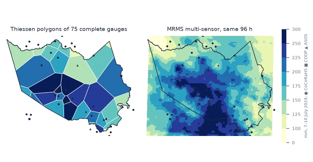
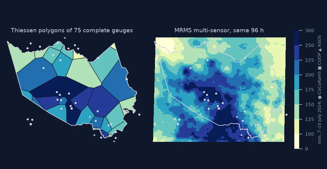
Who reported, storm sums, how far the network reaches
1. Find out who actually reported
GHCN-Daily mixes three networks around Houston: CoCoRaHS volunteers (station IDs beginning US1), the NWS Cooperative Observer Program (USC), and airport ASOS stations (USW). Count, per network, how many reported every day:
net = daily.index.get_level_values("STATION").str[:3].map({"US1": "CoCoRaHS", "USC": "COOP", "USW": "ASOS"})
summary = pd.DataFrame({"network": net, "days": daily.notna().sum(axis=1).values})
print(summary.groupby("network").days.agg(gauges="size", all_4_days=lambda d: (d == 4).sum(),
                                          missing_any=lambda d: (d < 4).sum()).to_string())
gauges all_4_days missing_any
network
ASOS 10 6 4
COOP 13 10 3
CoCoRaHS 158 59 99
Most gauges skipped at least one day around the storm, and nearly all of the gaps are among volunteers. A sum over the days a gauge did report would understate the storm wherever a report is missing, so incomplete gauges are left out here. The cost is density.
2. Sum over the storm, not over a day
The networks close their day at different times. ASOS stations use midnight-to-midnight local standard time; most CoCoRaHS and many COOP observers read the gauge at 7 am and date the reading that morning. The same rain lands on different dates:
iah = daily.xs("USW00012960", level="STATION").iloc[0]
coco = daily.loc[daily.index.get_level_values("STATION").str.startswith("US1")].dropna()
print("IAH (ASOS):", iah.to_dict())
print("CoCoRaHS median by date:", coco.median().round(1).to_dict())
IAH (ASOS): {'2024-07-07': 8.1, '2024-07-08': 119.9, '2024-07-09': 0.0, '2024-07-10': 0.0}
CoCoRaHS median by date: {'2024-07-07': 1.0, '2024-07-08': 75.4, '2024-07-09': 64.3, '2024-07-10': 0.0}
At the airport Beryl's rain is all on 8 July. The volunteers' median splits it, 75 mm on 8 July and 64 mm on 9 July: Beryl's rain began overnight, so a 7 am reading on the 8th caught the first part and the next morning's reading the rest. A four-day storm total does not care where each network draws its line, and its MRMS counterpart — 24 hours ending 12 UTC 7 July plus 72 hours ending 12 UTC 10 July — covers the same 96 hours as the 7 am observers.
3. Measure how far the network has to stretch
Within a county, how far is any point from its nearest complete gauge?
xmin, ymin, xmax, ymax = HARRIS.bounds
xx, yy = np.meshgrid(np.arange(xmin, xmax, 500), np.arange(ymin, ymax, 500))
grid = gpd.GeoSeries(gpd.points_from_xy(xx.ravel(), yy.ravel()), crs=32615)
grid = grid[grid.within(HARRIS)]
dist, _ = cKDTree(np.c_[g.geometry.x, g.geometry.y]).query(np.c_[grid.x, grid.y])
print(f"{len(inside)} complete gauges inside: one per {HARRIS.area / 1e6 / len(inside):.0f} km2")
print(f"distance to the nearest gauge: median {np.median(dist) / 1000:.1f} km, 90th percentile "
      f"{np.percentile(dist, 90) / 1000:.1f} km, max {dist.max() / 1000:.1f} km; "
      f"{(dist > 5000).mean():.0%} of the county is more than 5 km from one")
20 complete gauges inside: one per 229 km2
distance to the nearest gauge: median 8.0 km, 90th percentile 15.3 km, max 23.9 km; 73% of the county is more than 5 km from one
Convective rain cells are a few kilometres across. Over most of the county, the nearest gauge is farther away than that.
4. Weight by area: arithmetic mean against Thiessen polygons
An arithmetic mean gives each gauge the same weight, so a cluster of volunteers in one suburb counts many times. Thiessen polygons give each gauge the area closer to it than to any other gauge:
print(f"{len(cells)} polygons cover the county; the largest {cells.km2.max():.0f} km2, the smallest {cells.km2.min():.2f} km2")
print(f"the 5 largest polygons carry {cells.km2.nlargest(5).sum() / cells.km2.sum():.0%} of the weight")
print(cells.nlargest(5, "km2")[["STATION", "mm", "km2"]].round(1).to_string(index=False))
35 polygons cover the county; the largest 524 km2, the smallest 0.08 km2
the 5 largest polygons carry 45% of the weight
STATION mm km2
US1TXHRR251 208.8 524.2
USC00410586 222.5 450.6
USW00012960 128.0 395.8
US1TXHRR093 235.4 377.5
US1TXHRR306 151.4 324.4
The weights are very uneven: a handful of isolated gauges carry much of the county. One broken gauge there would move the county total far more than the same fault in a dense suburb.
Does the network see what MRMS sees
The data used on this page
GHCN-Daily precipitation, 7–10 July 2024, for every station in the GHCN-Daily inventory between 28.8–30.4°N and 94.6–96.3°W, from the NCEI daily-summaries service; MRMS MultiSensor QPE Pass 2, 24 h ending 12 UTC 7 July and 72 h ending 12 UTC 10 July 2024, from the NOAA MRMS archive on AWS; the US Census cartographic boundary file for counties, 2023.
import gzip
import shutil
from pathlib import Path

import geopandas as gpd
import numpy as np
import pandas as pd
import requests
import xarray as xr
from scipy.spatial import cKDTree
from shapely.geometry import MultiPoint
from shapely.ops import voronoi_diagram

Path("data").mkdir(exist_ok=True)


def fetch(url, name):
    if not Path("data", name).exists():
        Path("data", name).write_bytes(requests.get(url, timeout=600).content)
    return Path("data", name)


inv = pd.read_fwf(fetch("https://www.ncei.noaa.gov/pub/data/ghcn/daily/ghcnd-inventory.txt", "ghcnd-inventory.txt"),
                  widths=[11, 9, 10, 5, 5, 5], names=["id", "lat", "lon", "el", "first", "last"])
ids = inv[(inv.el == "PRCP") & (inv["last"] >= 2024) & inv.lat.between(28.8, 30.4) & inv.lon.between(-96.3, -94.6)].id.unique()
if not Path("data/gauges.csv").exists():
    parts = []
    for i in range(0, len(ids), 90):
        text = requests.get("https://www.ncei.noaa.gov/access/services/data/v1", timeout=300, params={
            "dataset": "daily-summaries", "dataTypes": "PRCP", "stations": ",".join(ids[i:i + 90]),
            "startDate": "2024-07-07", "endDate": "2024-07-10", "format": "csv", "includeStationLocation": 1,
            "units": "metric"}).text
        parts.append(text if not parts else text.split("\n", 1)[1])
    Path("data/gauges.csv").write_text("".join(parts))
raw = pd.read_csv("data/gauges.csv")
daily = raw.pivot_table(index=["STATION", "LATITUDE", "LONGITUDE"], columns="DATE", values="PRCP")

def mrms(product, stamp):
    name = f"MRMS_{product}_00.00_{stamp}.grib2"
    gz = fetch(f"https://noaa-mrms-pds.s3.amazonaws.com/CONUS/{product}_00.00/{stamp[:8]}/{name}.gz", name + ".gz")
    if not Path("data", name).exists():
        with gzip.open(gz) as src, open(Path("data", name), "wb") as dst:
            shutil.copyfileobj(src, dst)
    q = xr.open_dataset(Path("data", name), engine="cfgrib", decode_timedelta=True, backend_kwargs={"indexpath": ""})["unknown"]
    return q.where(q >= 0)

MRMS_96H = mrms("MultiSensor_QPE_24H_Pass2", "20240707-120000") + mrms("MultiSensor_QPE_72H_Pass2", "20240710-120000")
counties = gpd.read_file(fetch("https://www2.census.gov/geo/tiger/GENZ2023/shp/cb_2023_us_county_500k.zip", "cb_2023_us_county_500k.zip"))
harris = counties[(counties.STATEFP == "48") & (counties.NAME == "Harris")]
HARRIS = harris.to_crs(32615).geometry.iloc[0]
box = MRMS_96H.sel(latitude=slice(30.2, 29.4), longitude=slice(264.0, 265.1))
lon, lat = np.meshgrid(box.longitude.values - 360, box.latitude.values)
in_county = gpd.GeoSeries(gpd.points_from_xy(lon.ravel(), lat.ravel()), crs=4326).within(harris.geometry.iloc[0]).values
MRMS_IN_HARRIS = pd.Series(box.values.ravel()[in_county]).dropna()
print(f"{len(ids)} stations listed, {len(daily)} with data; MRMS: {len(MRMS_IN_HARRIS):,} cells in Harris County")
241 stations listed, 181 with data; MRMS: 4,283 cells in Harris County
Example 1: does the network see what MRMS sees?
Sample the MRMS field at the gauge locations and average it the same two ways. If that reproduces the full-field county mean, the network's layout is good enough for this storm, and any difference between gauges and MRMS is about measurement, not sampling:
gl = g.to_crs(4326)
g["mrms"] = MRMS_96H.sel(latitude=xr.DataArray(gl.geometry.y.values, dims="p"),
                         longitude=xr.DataArray(gl.geometry.x.values % 360, dims="p"), method="nearest").values
cells = cells.merge(g[["STATION", "mrms"]], on="STATION")
print(f"MRMS county mean from every cell: {MRMS_IN_HARRIS.mean():.1f} mm")
print(f"MRMS sampled at the gauges: arithmetic {g.loc[inside.index, 'mrms'].mean():.1f} mm, "
      f"Thiessen {(cells.mrms * cells.km2).sum() / cells.km2.sum():.1f} mm")
print(f"gauge against MRMS at the same points: r = {np.corrcoef(g.mm, g.mrms)[0, 1]:.2f}, "
      f"median gauge/MRMS {(g.mm / g.mrms).median():.2f}")
MRMS county mean from every cell: 188.9 mm
MRMS sampled at the gauges: arithmetic 211.9 mm, Thiessen 188.5 mm
gauge against MRMS at the same points: r = 0.76, median gauge/MRMS 1.04
The Thiessen weighting is what makes the network work. Sampled at the gauges, MRMS's arithmetic mean is 23 mm too high — the same bias as the gauges' own arithmetic mean in the quick answer — because volunteers cluster where it rained hardest. Weighted by area, the same samples land within half a millimetre of the full field. What is left between the gauges' 198.8 mm and MRMS's 188.9 mm is measurement: gauges caught about 4% more than MRMS at the same points.
Example 2: how many gauges does a county mean need?
rng = np.random.default_rng(42)
field = MRMS_IN_HARRIS.values
for n in sorted({5, 10, len(inside), 50, 100}):
    errors = [field[rng.choice(len(field), n, replace=False)].mean() - field.mean() for _ in range(500)]
    print(f"{n:3d} randomly placed gauges: county-mean error sd {np.std(errors):4.1f} mm "
          f"({np.std(errors) / field.mean():.1%})")
5 randomly placed gauges: county-mean error sd 20.0 mm (10.6%)
10 randomly placed gauges: county-mean error sd 13.6 mm (7.2%)
20 randomly placed gauges: county-mean error sd 9.9 mm (5.2%)
50 randomly placed gauges: county-mean error sd 5.9 mm (3.1%)
100 randomly placed gauges: county-mean error sd 4.0 mm (2.1%)
The real network of 20 complete gauges, Thiessen-weighted, came within 0.4 mm of MRMS's own mean — closer than the 9.9 mm typical of 20 random gauges, partly by luck. Randomly placed gauges are an idealisation — real ones cluster where people live — but the scaling holds: halving the error takes four times the gauges.
A sample of a field that varies at every scale
A gauge network is a sample of a field that varies at every scale. Three things decide how well it represents an area. Completeness: a missing report is a hole, not a zero. Alignment: networks with different observation times split the same storm across different days, so totals must be built over windows that every network covers whole. Geometry: the spacing of the gauges against the size of the rain cells, and how the gauges are weighted.
For a whole-county storm total, this network does well — but only when weighted by area. Sampled at the gauges, MRMS gives 188.5 mm by Thiessen polygons against 188.9 mm over every cell; the arithmetic mean of the same samples gives 211.9 mm, because the gauges cluster in the wetter parts of the county. What the network cannot do is resolve the field. Over much of Harris County the nearest complete gauge is several kilometres away, so a local downpour between gauges goes unseen. That is why rainfall products such as MRMS combine the gauges' absolute accuracy with radar's spatial detail. It is also why one gauge's total at one address says little about the next street.
Thiessen polygons, edges and multi-day reports
- Thiessen polygons ignore everything but distance; inverse-distance weighting or kriging smooth the field instead of stepping it.
- Polygons at the edge come from gauges outside the area; include neighbours before clipping, as here.
- Gauge undercatch grows with wind speed and is worst for unshielded gauges, so a hurricane's gauge totals lean low.
- CoCoRaHS multi-day reports (after a weekend) arrive as one accumulated value; GHCN flags them.
- Harris County Flood Control District runs a much denser real-time gauge network that is not in GHCN-Daily.
- Coordinates of volunteer gauges are often rounded; snap carefully before matching to a radar grid.
Internal links
- How to compare radar rainfall with gauges — matching windows, gauge by gauge
- Rainfall totals come out wrong — missing hours and false zeros
- How to map storm-total rainfall — county totals from MRMS
- Voronoi service areas in Python — the same geometry
- Spatial interpolation explained — beyond Thiessen
FAQ
What is the Thiessen polygon method for rainfall?
Each gauge is assigned the area closer to it than to any other gauge, and the areal rainfall is the area-weighted mean of the gauge values.
Why do neighbouring rain gauges disagree on which day it rained?
Networks end their day at different times: ASOS at local midnight, most CoCoRaHS and COOP observers at about 7 am. Sum over the whole storm to compare them.
How dense should a rain gauge network be?
It depends on the use. For a county-mean storm total a few dozen gauges can be enough; to resolve convective cells you need spacing of a few kilometres, which only radar provides everywhere.
Should I include gauges with missing days?
Not in a sum: a missing day is not a dry day. Use only complete gauges, or fill gaps from a radar-gauge product and say so.