How to Read NEXRAD Level II Radar Data in Python

Problem statement

The US weather radar network, NEXRAD, has published every volume scan from its 160 radars since the 1990s, and the full-resolution Level II archive is free on AWS. A single file holds a complete picture of the atmosphere around one radar in five to ten minutes: reflectivity, velocity and dual-polarisation fields on a stack of tilted cones. It is also an unusual data structure — polar coordinates, sweeps at repeated angles with different fields, ranges that differ between sweeps — and code written for ordinary rasters gets it wrong.

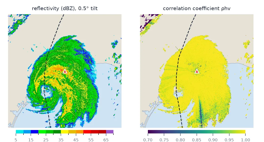
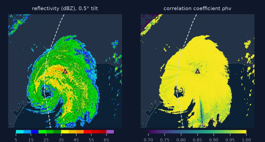
This page reads the KHGX (Houston/Galveston) volume from 09:01 UTC on 8 July 2024, minutes after Hurricane Beryl made landfall near Matagorda, Texas, with xradar, and explains what is in it.

Quick answer

List the volumes for a radar and hour in the public bucket, download one, and open it as a tree of sweeps:

listing = requests.get(BUCKET, params={"list-type": 2, "prefix": "2024/07/08/KHGX/KHGX20240708_09"}, timeout=60).text
keys = [k for k in re.findall(r"<Key>([^<]+)</Key>", listing) if not k.endswith("_MDM")]
print(len(keys), "volumes in the hour; first:", keys[0])
path = fetch(keys[0])
dt = xd.io.open_nexradlevel2_datatree(path)
sweeps = [(name, round(float(dt[name].ds.sweep_fixed_angle), 2)) for name in dt.children]
print(len(sweeps), "sweeps; elevation angles:", [a for _, a in sweeps])

9 volumes in the hour; first: 2024/07/08/KHGX/KHGX20240708_090125_V06
23 sweeps; elevation angles: [0.48, 0.48, 0.88, 0.88, 0.48, 0.48, 1.32, 1.32, 1.8, 0.48, 0.48, 2.42, 3.12, 4.0, 5.1, 6.42, 0.48, 0.48, 8.0, 10.02, 12.48, 15.6, 19.51]

Find the file, read the volume, match sweeps to fields

1. Find the file

The Unidata NEXRAD Level II archive on AWS is organised as YYYY/MM/DD/SITE/SITEYYYYMMDD_HHMMSS_V06. Files ending _MDM are metadata, not scans. A listing request with a prefix returns the keys for any hour:

print(keys[:3])
print(round(Path(path).stat().st_size / 1e6, 1), "MB for one volume")

['2024/07/08/KHGX/KHGX20240708_090125_V06', '2024/07/08/KHGX/KHGX20240708_090818_V06', '2024/07/08/KHGX/KHGX20240708_091511_V06']
19.4 MB for one volume

2. Read the station and the volume

Each file is one volume scan: the radar sweeps a full circle at one elevation, tilts up, and repeats, from 0.5° to 19.5° in this storm-mode scan, with extra low-level passes inserted along the way (Example 2). The root of the tree holds the station:

root = dt.ds
print(root.attrs.get("instrument_name"), f"{float(root.latitude):.4f} N, {float(root.longitude):.4f} E, {float(root.altitude):.0f} m")

KHGX 29.4719 N, -95.0787 E, 34 m

3. Know which sweep carries which field

Low tilts are scanned twice: once in long-range "surveillance" mode for reflectivity and dual-polarisation fields, once in short-range "Doppler" mode for velocity. So sweep 0 and sweep 1 have the same angle and different variables and ranges:

for name in list(dt.children)[:4]:
    s = dt[name].ds
    fields = [k for k in s.data_vars if s[k].ndim == 2]
    print(f"{name}: {float(s.sweep_fixed_angle):.2f} deg, {s.azimuth.size} rays x {s.range.size} gates "
          f"to {float(s.range.max()) / 1000:.0f} km, fields {fields}")

sweep_0: 0.48 deg, 720 rays x 1832 gates to 460 km, fields ['DBZH', 'ZDR', 'PHIDP', 'RHOHV', 'CCORH']
sweep_1: 0.48 deg, 720 rays x 1192 gates to 300 km, fields ['DBZH', 'VRADH', 'WRADH']
sweep_2: 0.88 deg, 720 rays x 1832 gates to 460 km, fields ['DBZH', 'ZDR', 'PHIDP', 'RHOHV', 'CCORH']
sweep_3: 0.88 deg, 720 rays x 1192 gates to 300 km, fields ['DBZH', 'VRADH', 'WRADH']

Code that picks "the 0.5° sweep" by angle alone gets whichever comes first; pick by angle and the field you need.

4. Read the polar grid

A sweep is a 2-D array indexed by azimuth and range. KHGX's super-resolution low tilts have 720 rays — one every half degree — and gates every 250 m:

sw = dt["sweep_0"].ds
print(f"first gate {float(sw.range[0]):.0f} m, spacing {float(sw.range[1] - sw.range[0]):.0f} m; "
      f"sweep took {(sw.time.max() - sw.time.min()).values / np.timedelta64(1, 's'):.0f} s")
print(f"reflectivity: max {float(sw.DBZH.max()):.0f} dBZ; share of gates within 200 km at 40 dBZ or more: "
      f"{float(((sw.DBZH >= 40) & (sw.range < 200_000)).sum() / ((sw.range < 200_000).sum() * sw.azimuth.size)):.0%}")

first gate 2125 m, spacing 250 m; sweep took 16 s
reflectivity: max 66 dBZ; share of gates within 200 km at 40 dBZ or more: 12%

5. Georeference

xradar adds Cartesian x, y and height for each gate, using the standard 4/3-Earth-radius beam propagation model. Height matters: at long range even the lowest beam is far above the ground:

geo = dt.xradar.georeference()["sweep_0"].ds
k = int(np.argmin(np.abs(geo.range.values - 130_000)))
print(f"beam centre at 130 km range, 0.48 deg tilt: {float(geo.z[0, k]):.0f} m above the radar's datum")

beam centre at 130 km range, 0.48 deg tilt: 2022 m above the radar's datum

Beryl's eye was about 124 km from KHGX at landfall; the radar was looking at it two kilometres up.

Picking sweeps from a Houston radar volume

The data used on this page

NOAA NEXRAD Level II, radar KHGX (Houston/Galveston, League City TX), volume 2024-07-08 09:01:25 UTC, from the Unidata NEXRAD Level II archive on AWS (NOAA Open Data Dissemination); track position from IBTrACS v04r01.

import re
from pathlib import Path

import numpy as np
import requests
import xradar as xd

BUCKET = "https://unidata-nexrad-level2.s3.amazonaws.com/"
Path("data").mkdir(exist_ok=True)

def fetch(key):
    path = Path("data") / key.split("/")[-1]
    if not path.exists():
        path.write_bytes(requests.get(BUCKET + key, timeout=300).content)
    return str(path)

print(BUCKET)

https://unidata-nexrad-level2.s3.amazonaws.com/

Example 1: pick a sweep by angle and field

def sweep_with(dt, angle, field, tol=0.2):
    for name in dt.children:
        s = dt[name].ds
        if abs(float(s.sweep_fixed_angle) - angle) < tol and field in s:
            return name
    raise KeyError(f"no {field} sweep near {angle} deg")

print("reflectivity at 0.5:", sweep_with(dt, 0.5, "DBZH"), "| velocity at 0.5:", sweep_with(dt, 0.5, "VRADH"))

reflectivity at 0.5: sweep_0 | velocity at 0.5: sweep_1

Example 2: the low tilt, again and again

In this volume the 0.48° tilt appears eight times. In severe weather NEXRAD radars run SAILS — supplemental adaptive intra-volume low-level scans — inserting extra low-level passes into the volume so forecasters get a fresh low-level view every minute or two:

low = [(n, str(dt[n].ds.time.min().values)[11:19], "DBZH" in dt[n].ds and "ZDR" in dt[n].ds, dt[n].ds.attrs.get("sails_cut"))
       for n in dt.children if abs(float(dt[n].ds.sweep_fixed_angle) - 0.48) < 0.1]
for name, t, dualpol, sails in low:
    print(f"{name:9} starts {t}  {'reflectivity + dual-pol' if dualpol else 'velocity'}  SAILS cut: {sails}")

sweep_0   starts 09:01:25  reflectivity + dual-pol  SAILS cut: False
sweep_1   starts 09:01:43  velocity  SAILS cut: False
sweep_4   starts 09:02:50  reflectivity + dual-pol  SAILS cut: True
sweep_5   starts 09:03:08  velocity  SAILS cut: True
sweep_9   starts 09:04:28  reflectivity + dual-pol  SAILS cut: True
sweep_10  starts 09:04:46  velocity  SAILS cut: True
sweep_16  starts 09:06:21  reflectivity + dual-pol  SAILS cut: True
sweep_17  starts 09:06:39  velocity  SAILS cut: True

For a single picture of the volume, use the first pair; for a low-level time series within one file, the repeats are a bonus.

How a weather radar measures

A weather radar sends pulses along a narrow beam and listens for echoes, timing them for range and measuring their strength for reflectivity, their Doppler shift for velocity and, with two polarisations, the shape of what reflected them. Rotating while tilting through a set of angles produces a volume of conical sweeps — the native data structure of every radar file.

Three features of that structure trip up first-time readers. Coordinates are polar, so nothing is on a rectangular grid until you put it there. Sweeps at the same angle can carry different fields, because the radar scans low tilts twice in different modes. And the beam rises with distance — partly from its tilt, partly from the Earth's curvature — so a "surface" reflectivity map is surface only near the radar. xradar keeps all of this explicit: one dataset per sweep, with angles, ranges, times and fields as they were recorded.

Metadata files, repeated tilts and velocity aliasing

• Skip _MDM files; they are metadata.
• Low tilts are repeated in surveillance and Doppler modes with different fields and ranges.
• Super-resolution gives 720 rays and 250 m gates on low tilts; higher tilts may have fewer.
• Beam height at 130 km is about 2 km on the lowest tilt.
• SAILS repeats the lowest tilt several times within one volume.
• Velocity aliasing must be corrected before velocities are trusted.
• Volumes take five to ten minutes; each sweep has its own time.

Internal links

• Weather radar reflectivity explained — what dBZ means
• How to grid radar data — from polar sweeps to a raster
• Dual-polarisation radar explained — ZDR and ρhv
• Radar beam blockage and clutter — what the beam runs into
• How to plot a hurricane track from IBTrACS — Beryl's path

FAQ

Where can I download NEXRAD Level II data?

From the Unidata NEXRAD Level II archive on AWS (unidata-nexrad-level2), organised by date and radar site, free and without an account.

How do I read NEXRAD Level II in Python?

xradar.io.open_nexradlevel2_datatree(path) returns a tree with one dataset per sweep; Py-ART's pyart.io.read_nexrad_archive is an alternative.

Why are there two sweeps at 0.5 degrees?

The radar scans low tilts once for reflectivity and dual-polarisation fields over a long range and once for velocity over a shorter range.

How high is the radar beam?

On the 0.5° tilt, about 2 km above the radar at 130 km range under the standard 4/3-Earth model, and higher with distance.