How to Analyse a Sea-Ice Extent Time Series in Python

Problem statement

The National Snow and Ice Data Center publishes the daily extent of Arctic and Antarctic sea ice since 1978 as a small CSV file, and it is the most quoted climate record there is. It is also easy to analyse badly. The file is not a clean daily series: for its first nine years it has a value every other day, there is a six-week hole in the winter of 1987–88, the most recent weeks come from a different satellite product and are revised, and the file changes every day it is downloaded. A trend, a record low or a "lowest since" claim computed without handling those will be wrong in ways that are hard to spot.

This page reads the NSIDC Sea Ice Index (G02135, version 4) daily extent for the Arctic, cleans it into a series you can compute with, and measures the September minimum, its trend and its ranking — with every number tied to a fixed end date so it reproduces.

Quick answer

Read the CSV, skip its units row, fix the end date, put it on a daily index, and work from monthly means for trends:

d = pd.read_csv("data/N_seaice_extent_daily_v4.0.csv", skiprows=[1], skipinitialspace=True)
d.columns = d.columns.str.strip()
d["date"] = pd.to_datetime(dict(year=d.Year, month=d.Month, day=d.Day))
s = d[(d.date >= "1979-01-01") & (d.date <= END)].set_index("date")["Extent"]
sept = s[s.index.month == 9].groupby(s[s.index.month == 9].index.year).mean()
slope = np.polyfit(sept.index, sept.values, 1)[0] * 10
base = sept.loc[1981:2010].mean()
print(f"September mean extent: 1979 {sept.loc[1979]:.2f}, 2012 {sept.loc[2012]:.2f}, 2025 {sept.loc[2025]:.2f} million km²")
print(f"trend {slope:+.2f} million km² per decade = {slope / base:+.1%} of the 1981-2010 mean per decade")

September mean extent: 1979 7.05, 2012 3.57, 2025 4.75 million km²
trend -0.76 million km² per decade = -11.9% of the 1981-2010 mean per decade

Read it as it is, find gaps, smooth as NSIDC does, rank minima

1. Read the file as it is

The first row is a header, the second a row of units, and the last column a list of source files, sometimes quoted, sometimes not. skiprows=[1] drops the units and skipinitialspace=True strips the padding the columns are aligned with:

print(d.columns.tolist())
print(d[["date", "Extent", "Missing"]].tail(3).to_string(index=False))
print("rows after", END, ":", int((d.date > END).sum()), "- excluded so the numbers reproduce")

['Year', 'Month', 'Day', 'Extent', 'Missing', 'Source Data', 'date']
      date  Extent  Missing
2026-09-27   5.228      0.0
2026-09-28   5.333      0.0
2026-09-29   5.337      0.0
rows after 2025-12-31 : 272 - excluded so the numbers reproduce

The file is regenerated every day with the newest values appended, and the last few weeks are near-real-time data from a different product. Fixing an end date — here the last day of 2025 — is what makes a result reproducible.

2. Find the gaps

gaps = s.index.to_series().diff().dt.days
print(gaps.value_counts().sort_index().to_string())
big = gaps[gaps > 2]
print("longest gap:", int(big.max()), "days, ending", big.idxmax().date())

date
1.0     13971
2.0      1576
42.0        1
longest gap: 42 days, ending 1988-01-13

Until August 1987 the record has a value every second day — the early satellite sensor observed on alternate days. Then there is a 42-day hole from December 1987 into January 1988 with no usable satellite data at all. Any statistic that assumes one value per day counts the 1980s at half weight.

3. Put it on a daily index and smooth as NSIDC does

daily = s.asfreq("D")
filled = daily.interpolate(limit=3)                     # bridge the alternate days, not the 1987-88 hole
five = filled.rolling(5).mean()                         # NSIDC quotes daily values as 5-day trailing means
print(f"missing days on the daily index: {daily.isna().sum():,}; still missing after filling gaps of up to 3 days: {filled.isna().sum()}")

missing days on the daily index: 1,617; still missing after filling gaps of up to 3 days: 38

4. Rank the minima

The annual minimum is usually in September. Rank years by their lowest 5-day mean:

minima = five.groupby(five.index.year).min()
dates = five.groupby(five.index.year).idxmin()
top = minima.loc[1979:].nsmallest(5)
for y, v in top.items():
    print(f"{y}: {v:.2f} million km² on {dates[y]:%d %B}")

2012: 3.39 million km² on 17 September
2020: 3.82 million km² on 16 September
2007: 4.15 million km² on 18 September
2016: 4.17 million km² on 10 September
2019: 4.19 million km² on 18 September

2012 remains the lowest in the record by a wide margin; the years that follow it are spread across the last two decades. A claim that a year was "the second lowest" depends on whether it is ranked by daily, 5-day or monthly values, so say which.

5. Measure the trend on monthly means

Daily values are autocorrelated and the early record is half-sampled; monthly means are neither. The September trend from the quick answer, and March for comparison:

mar = s[s.index.month == 3].groupby(s[s.index.month == 3].index.year).mean()
for label, series in (("March (maximum)", mar), ("September (minimum)", sept)):
    b = np.polyfit(series.index, series.values, 1)[0] * 10
    print(f"{label:20} {b:+.2f} million km² per decade ({b / series.loc[1981:2010].mean():+.1%} of 1981-2010 per decade)")

March (maximum)      -0.38 million km² per decade (-2.5% of 1981-2010 per decade)
September (minimum)  -0.76 million km² per decade (-11.9% of 1981-2010 per decade)

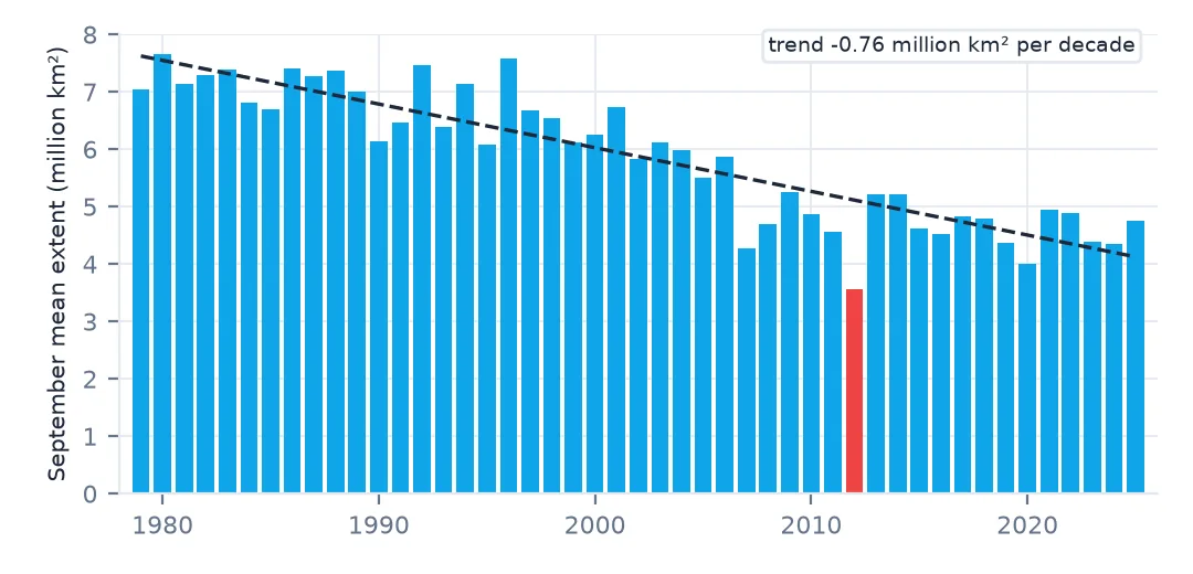
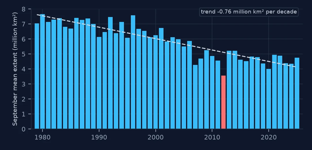
The summer minimum is shrinking twice as fast as the winter maximum in absolute terms, and almost five times as fast relative to its own average — which is why the September record is the one usually shown.

A climatology band like NSIDC's chart

The data used on this page

NSIDC Sea Ice Index, version 4 (G02135), daily extent for the Northern Hemisphere, from NSIDC / NOAA at noaadata.apps.nsidc.org. Fetterer, F., K. Knowles, W. N. Meier, M. Savoie, and A. K. Windnagel. Sea Ice Index, Version 4. Boulder, Colorado USA. NSIDC: National Snow and Ice Data Center. Values used here end on 31 December 2025.

from pathlib import Path

import numpy as np
import pandas as pd
import requests

Path("data").mkdir(exist_ok=True)
UA = {"User-Agent": "spatialworkflow.io guide (https://www.spatialworkflow.io)"}
URL = "https://noaadata.apps.nsidc.org/NOAA/G02135/north/daily/data/N_seaice_extent_daily_v4.0.csv"
if not Path("data/N_seaice_extent_daily_v4.0.csv").exists():
    Path("data/N_seaice_extent_daily_v4.0.csv").write_bytes(requests.get(URL, headers=UA, timeout=120).content)
END = "2025-12-31"                                       # fixed, so the numbers on this page reproduce
print(Path("data/N_seaice_extent_daily_v4.0.csv").stat().st_size > 1_000_000)

True

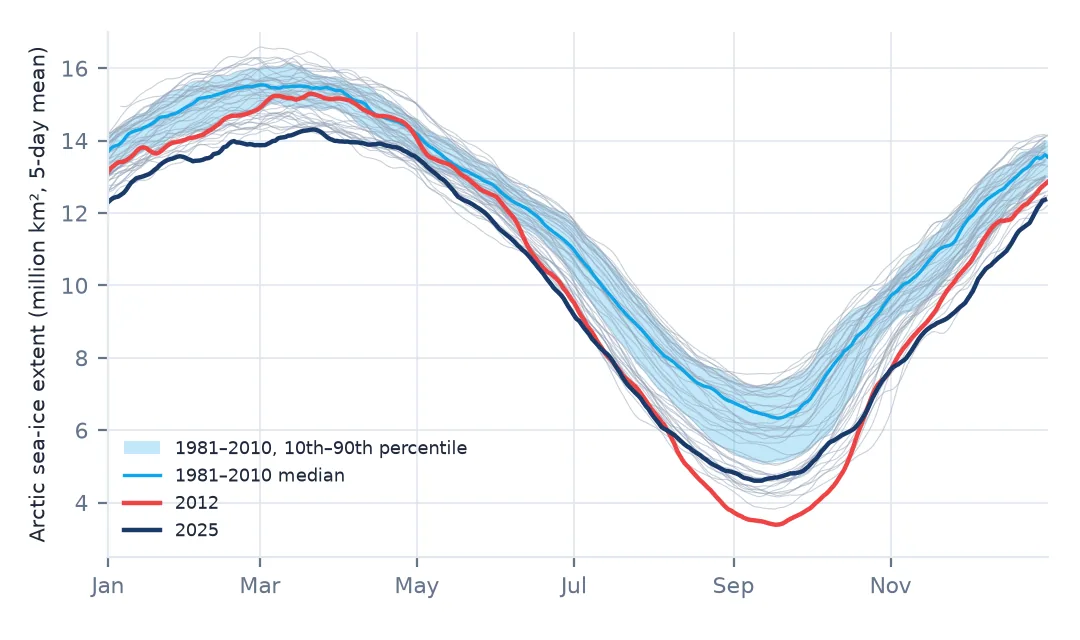
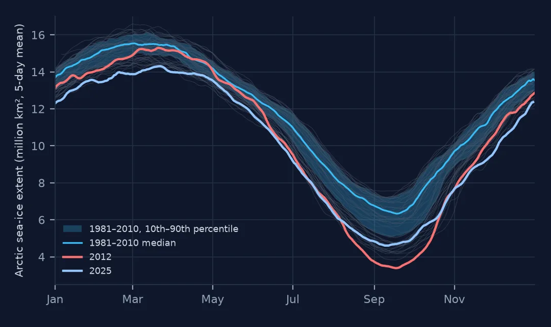
Example 1: a climatology band, the way the NSIDC chart draws it

The familiar chart shows each year against the 1981–2010 median and interdecile range by day of year:

doy = five.index.dayofyear
clim = five[(five.index.year >= 1981) & (five.index.year <= 2010)]
band = clim.groupby(clim.index.dayofyear).quantile([0.1, 0.5, 0.9]).unstack()
y25 = five["2025"]
below = (y25.values < band.loc[y25.index.dayofyear, 0.1].values).mean()
print(f"2025 days below the 1981-2010 10th percentile: {below:.0%}")
print(band.loc[[60, 258]].round(2).rename(index={60: "1 March", 258: "15 September"}).to_string())

2025 days below the 1981-2010 10th percentile: 100%
                0.1    0.5    0.9
date                             
1 March       14.83  15.53  16.03
15 September   5.10   6.39   7.26

Example 2: how much the smoothing and the sampling change a record

raw_min = s.groupby(s.index.year).min().loc[1979:2025]
print("lowest raw daily value:", raw_min.idxmin(), round(raw_min.min(), 3))
print("lowest 5-day mean:     ", minima.loc[1979:].idxmin(), round(minima.loc[1979:].min(), 3))
early = minima.loc[1979:1986]
print(f"1979-86 minima from alternate-day data, interpolated: mean {early.mean():.2f} million km²")

lowest raw daily value: 2012 3.34
lowest 5-day mean:      2012 3.387
1979-86 minima from alternate-day data, interpolated: mean 6.98 million km²

Smoothing raises every minimum slightly and can reorder close years; quote the method with the number.

What extent counts

Sea-ice extent is the total area of grid cells with at least 15% ice concentration — a threshold count, not the area of ice itself (see sea-ice extent versus area). The daily series is computed from passive microwave satellites flown since late 1978, and the record stitches several sensors together; the alternate-day sampling and the 1987–88 gap are the seams that show.

Three habits keep an analysis honest. Fix the end date, because the file changes daily and its newest values are provisional. Handle the sampling explicitly — a daily index with short gaps filled, the long gap left empty — rather than letting a groupby silently average over unequal numbers of days. And compute trends on monthly means, which are the quantities the record's producers themselves trend, and report the trend both in absolute terms and relative to a stated baseline.

Daily updates, early alternate days and the 1987-88 hole

• The file updates daily. Fix an end date and record the download date.
• Every other day until August 1987. Interpolate short gaps; do not count days.
• The 1987–88 hole is 42 days; leave it missing.
• 5-day trailing means are the NSIDC convention for daily values.
• Monthly means for trends; daily values are autocorrelated.
• Antarctic ice behaves differently; the southern file is analysed the same way but tells a different story.

Internal links

• Sea-ice extent versus area explained — what the number measures
• How to map sea-ice concentration — the grids behind the totals
• Sea-ice extent numbers disagree — when two sources differ
• Polar stereographic projections explained — the grid the data are on
• Snow water equivalent explained — the other half of the cryosphere record

FAQ

Where can I download Arctic sea-ice extent data?

The NSIDC Sea Ice Index (G02135) publishes daily and monthly extent as CSV files for both hemispheres, free and without registration.

How fast is Arctic sea ice declining?

In this record, the September mean extent declined by about 0.76 million km² per decade from 1979 to 2025, about 12% of the 1981–2010 average per decade.

Why does the sea-ice record have missing days?

Until August 1987 the satellite instrument observed every other day, and from December 1987 to January 1988 there are 42 days with no usable data.

What was the lowest Arctic sea-ice extent?

September 2012 holds the record in this series, with a 5-day mean minimum of 3.39 million km².