
How to Animate Arctic Sea Ice Decline in Python
On this page
Problem statement
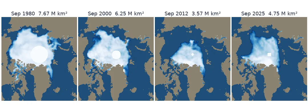
Arctic sea ice reaches its minimum each September, and the September minimum has shrunk since satellite records began in 1978. An animation of 47 Septembers makes that decline visible in a way a line chart cannot, because it shows where the ice went. The NSIDC Sea Ice Index publishes a concentration grid for every month, so the frames are easy to get. Getting them right is harder. The grid stores ice as coded integers. The hole around the pole shrinks twice as satellites change, which looks like ice appearing. And a naive extent calculation is wrong by up to 1.3 million km².
This page animates the September ice from 1979 to 2025 and checks every frame's extent against NSIDC's official numbers.
Quick answer
Read each September concentration GeoTIFF, mask the flag values, draw with a fixed colour scale, and label each frame with the official extent:
frames = []
for year in YEARS:
    a = conc(year)                                        # 0-100 % ice, NaN over land and coast, 100 in the pole hole
    fig, ax = plt.subplots(figsize=(4.5, 5), dpi=80)
    ax.imshow(LAND, cmap=LAND_CMAP, extent=EXTENT)
    ax.imshow(np.where(a >= 15, a, np.nan), cmap="Blues_r", vmin=15, vmax=100, extent=EXTENT)
    ax.set_xlim(-2.6e6, 2.6e6); ax.set_ylim(-3.2e6, 2.6e6); ax.set_axis_off()
    ax.set_title(f"September {year}   {official.loc[year, 'extent']:.2f} million km²", fontsize=10)
    fig.canvas.draw(); frames.append(np.asarray(fig.canvas.buffer_rgba())[..., :3].copy()); plt.close(fig)
iio.imwrite("data/sea_ice_september.gif", frames, duration=[300] * (len(frames) - 1) + [2000], loop=0)
print(f"{len(frames)} frames, {Path('data/sea_ice_september.gif').stat().st_size / 1e6:.2f} MB")
47 frames, 1.48 MB
Decode the grid, handle the pole hole, check extent
1. Decode the grid
The Sea Ice Index GeoTIFFs are 25 km cells on the NSIDC polar stereographic grid (EPSG:3411). Values 0 to 1000 are concentration in tenths of a percent; values above 1000 are flags:
with rasterio.open(tif(2024)) as r:
    raw = r.read(1)
    print(r.crs, r.res, r.shape)
vals, n = np.unique(raw[raw > 1000], return_counts=True)
print(dict(zip(vals.tolist(), n.tolist())), "— 2510 pole hole, 2530 coast, 2540 land")
print(f"ice concentration range {raw[raw <= 1000].min() / 10:.0f}–{raw[raw <= 1000].max() / 10:.0f} %")
EPSG:3411 (25000.0, 25000.0) (448, 304)
{2510: 44, 2530: 5052, 2540: 63212} — 2510 pole hole, 2530 coast, 2540 land
ice concentration range 0–100 %
2. Handle the pole hole
The satellites cannot see the area right around the pole, and how much they miss depends on the instrument. Count the hole in every year:
hole = pd.Series({y: int((read(y) == 2510).sum()) for y in YEARS})
for size, years in hole.groupby(hole).groups.items():
    print(f"{size:>5} cells ({size * 625:>9,} km²): {min(years)}–{max(years)}")
44 cells ( 27,500 km²): 2008–2024
96 cells ( 60,000 km²): 2025–2025
468 cells ( 292,500 km²): 1987–2007
1799 cells (1,124,375 km²): 1979–1986
In a raw animation the grey hole shrinks suddenly in 1987 and 2008, which reads as ice appearing at the pole. The area around the pole is ice-covered in September, and NSIDC counts the hole as ice when computing extent. Draw it as full ice too, or with a fixed hatching that every frame shares.
3. Check extent against the official numbers
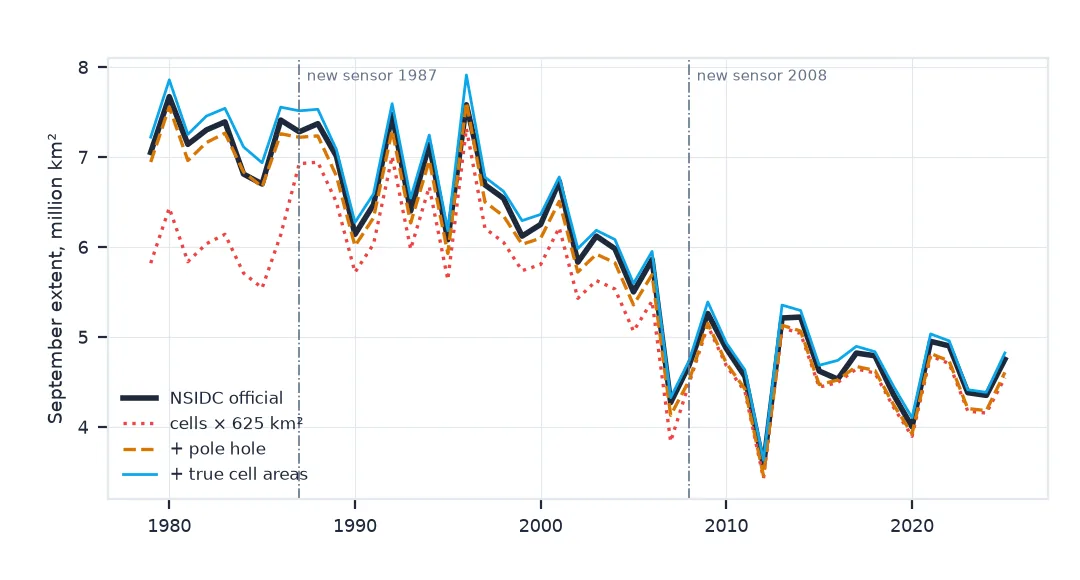
Extent is the area of all cells with at least 15% ice. Three corrections stand between a first attempt and NSIDC's number. Add them one at a time:
rows = []
for y in YEARS:
    a = read(y)
    ice, pole = (a >= 150) & (a <= 1000), a == 2510
    rows.append({"year": y, "cells x 625 km²": ice.sum() * 625 / 1e6,
                 "+ pole hole": (ice | pole).sum() * 625 / 1e6,
                 "+ true cell areas": CELL_KM2[ice | pole].sum() / 1e6})
mine = pd.DataFrame(rows).set_index("year")
err = mine.sub(official.extent, axis=0)
print(err.agg(["mean", "min", "max"]).round(2).to_string())
cells x 625 km² + pole hole + true cell areas
mean -0.47 -0.13 0.12
min -1.30 -0.22 0.03
max -0.04 0.03 0.33
CELL_KM2 is each cell's real area: a polar stereographic grid is true to scale only at 70° N, so a nominal 625 km² cell covers more ground near the pole and less towards the edges. With all three corrections the extent is consistently above the official one. That last gap comes from how the monthly number is made. NSIDC averages the daily extents, while this file holds the month's average concentration, and a cell that was ice-covered on only some days can still average 15%. Check it for one month:
daily = [CELL_KM2[((d >= 150) & (d <= 1000)) | (d == 2510)].sum() / 1e6 for d in map(read_daily, DAYS)]
print(f"September 2024: mean of {len(daily)} daily extents {np.mean(daily):.3f}, official {official.loc[2024, 'extent']}, "
      f"from the monthly grid {mine.loc[2024, '+ true cell areas']:.3f} million km²")
September 2024: mean of 30 daily extents 4.351, official 4.35, from the monthly grid 4.384 million km²
4. Put the trend in numbers
The animation shows the decline; the official series measures it:
slope = np.polyfit(official.index, official.extent, 1)[0]
low = official.extent.nsmallest(3)
print(f"trend {slope * 10:+.2f} million km² per decade ({slope * 10 / official.extent.iloc[:10].mean():+.1%} of the 1979–88 mean)")
print("lowest Septembers:", ", ".join(f"{y} ({v:.2f})" for y, v in low.items()))
trend -0.76 million km² per decade (-10.5% of the 1979–88 mean)
lowest Septembers: 2012 (3.57), 2020 (4.00), 2007 (4.27)
Frame extents beside the official series
The data used on this page
The NSIDC Sea Ice Index, version 4 (G02135): monthly September concentration GeoTIFFs for 1979–2025, the daily GeoTIFFs for September 2024, and the official monthly extent table.
from pathlib import Path

import imageio.v3 as iio
import matplotlib
matplotlib.use("Agg")
import matplotlib.pyplot as plt
import numpy as np
import pandas as pd
import pyproj
import rasterio
import requests
from matplotlib.colors import ListedColormap

BASE = "https://noaadata.apps.nsidc.org/NOAA/G02135/north"
D = Path("data/seaice"); D.mkdir(parents=True, exist_ok=True)
YEARS = range(1979, 2026)
DAYS = pd.date_range("2024-09-01", "2024-09-30")


def fetch(url, path):
    if not path.exists():
        path.write_bytes(requests.get(url, timeout=120).content)
    return path


tif = lambda y: fetch(f"{BASE}/monthly/geotiff/09_Sep/N_{y}09_concentration_v4.0.tif", D / f"N_{y}09_concentration_v4.0.tif")
read = lambda y: rasterio.open(tif(y)).read(1)
read_daily = lambda d: rasterio.open(fetch(f"{BASE}/daily/geotiff/{d:%Y}/{d:%m_%b}/N_{d:%Y%m%d}_concentration_v4.0.tif",
                                           D / f"d_N_{d:%Y%m%d}_concentration_v4.0.tif")).read(1)
official = pd.read_csv(fetch(f"{BASE}/monthly/data/N_09_extent_v4.0.csv", D / "N_09_extent_v4.0.csv"), skipinitialspace=True)
official.columns = official.columns.str.strip()
official = official.set_index("year").loc[:2025]  # the table gains a row each October


def conc(y):
    a = read(y).astype(float)
    out = np.where(a <= 1000, a / 10, np.nan)
    out[a == 2510] = 100.0                                 # pole hole: ice-covered, and counted as ice by NSIDC
    return out


with rasterio.open(tif(2024)) as r:
    T, (h, w) = r.transform, r.shape
    EXTENT = (T.c, T.c + w * T.a, T.f + h * T.e, T.f)
rows, cols = np.meshgrid(np.arange(h), np.arange(w), indexing="ij")
x, y = rasterio.transform.xy(T, rows.ravel(), cols.ravel())
lon, lat = pyproj.Transformer.from_crs(3411, 4326, always_xy=True).transform(np.array(x), np.array(y))
CELL_KM2 = (625 / pyproj.Proj("EPSG:3411").get_factors(lon, lat).areal_scale).reshape(h, w)
LAND = np.where(read(2024) >= 2530, 1.0, np.nan)
LAND_CMAP = ListedColormap(["#8a8170"])
print(f"{len(YEARS)} Septembers; cell areas {CELL_KM2.min():.0f}–{CELL_KM2.max():.0f} km² (nominal 625)")
47 Septembers; cell areas 383–664 km² (nominal 625)
Example 1: extent from each frame next to the official series
fig, ax = plt.subplots(figsize=(7, 3.5))
ax.plot(official.index, official.extent, "k-", lw=2, label="NSIDC official")
for col, style in zip(mine.columns, (":", "--", "-")):
    ax.plot(mine.index, mine[col], style, lw=1, label=col)
ax.set_ylabel("September extent, million km²"); ax.legend(fontsize=8)
fig.savefig("data/extent_check.png", dpi=150, bbox_inches="tight")
jumps = err["cells x 625 km²"].diff().loc[[1987, 2008]]
print("step in the naive error when the pole hole shrank:", jumps.round(2).to_dict())
step in the naive error when the pole hole shrank: {1987: 0.92, 2008: 0.23}
A fixed palette and the grid's conventions
A sea-ice animation is a raster animation with a fixed palette, and most of the work is the grid's conventions. Flags must not be drawn as concentrations; 2540 decoded as 254% ice paints the continents. The pole hole is an artefact of the satellite's orbit, not of the ice, and it changes with the satellite, so it has to look the same in every frame. And a single number on each frame invites comparison with NSIDC's published figure, so the number should be NSIDC's or agree with it.
The extent checks are what make the frame labels trustworthy. A cell count times 625 km² is off by up to 1.3 million km², more than the difference between many pairs of years. It is also off by different amounts before and after each sensor change. A trend computed that way would partly measure the satellites. With the pole hole and true cell areas included, the remaining difference is the monthly-mean method, and the daily files confirm it: their mean reproduces the official September 2024 figure.
Versions, recent years and coastal flags
- Version: these are version 4 files (
_v4.0); earlier versions give slightly different numbers, so say which one you used. - 2025 comes from a different source dataset (the extent table lists NSIDC-0803 instead of NSIDC-0051), and its pole hole is a new size again.
- Concentration below 15% is noise near the ice edge; do not draw it.
- Land and coast flags (2530, 2540) come from the grid, so coastlines are 25 km steps; draw a vector coastline on top for print.
- Southern hemisphere files use a different grid (EPSG:3412) and have no pole hole.
- Frame timing: hold the last frame longer (2 seconds here) so the latest year can be read.
Internal links
- How to make a drought monitor animation — checking each frame against official statistics
- How to make a GOES satellite loop — another satellite raster animation
FAQ
Where do I get Arctic sea ice data for Python?
The NSIDC Sea Ice Index (G02135) publishes daily and monthly concentration and extent GeoTIFFs on the polar stereographic grid, plus CSV tables of official extent, over plain HTTPS.
How is sea ice extent calculated?
It is the total area of grid cells with at least 15% ice concentration, counting the pole hole as ice and using each cell's true area. NSIDC's monthly figure is the average of the daily extents.
Why does my sea ice extent not match NSIDC?
Usually because the pole hole is left out or every cell is taken as 625 km². Once both are fixed, a remaining small excess comes from using the monthly concentration grid instead of averaging daily extents.
Why does the hole at the North Pole change size?
It is the area the satellite cannot see, and it depends on the instrument: it shrank in 1987 and 2008 as new sensors took over, and changed again in 2025.