
How to Compute Glacier Hypsometry from a DEM in Python
On this page
Problem statement
A glacier's hypsometry — how its area is distributed with elevation — decides how it responds to climate. A glacier with most of its area high up keeps a large accumulation zone when the snow line rises; one with a long low tongue loses area fast. Computing hypsometry is simple in principle: overlay a glacier outline on an elevation model and count area per elevation band. In practice the outline and the DEM come from different years, the DEM's cells are in degrees, and an outline from 1850 sits over a surface measured a century and a half later.
This page computes the hypsometry of the Great Aletsch Glacier, the largest in the Alps, from GLIMS outlines for 1850, 1973 and 2017 and the Copernicus 30 m DEM, and measures where the 27 km² it lost in between came from.
Quick answer
Reproject the DEM to an equal-area metric grid, rasterise each outline onto it, and histogram the elevations:
with rasterio.open("data/aletsch_dem_2056.tif") as src:
    z, tr, res = src.read(1), src.transform, src.res[0]
bands = np.arange(1400, 4300, 100)
hyps = {}
for year in (1850, 1973, 2017):
    geom = outlines.loc[outlines.year == year, "geometry"].iloc[0]
    inside = rasterize([(geom, 1)], out_shape=z.shape, transform=tr, dtype="uint8").astype(bool)
    hyps[year] = pd.Series(np.histogram(z[inside], bins=bands)[0] * res * res / 1e6, index=bands[:-1])
h = pd.DataFrame(hyps)
print(h.sum().round(1).to_dict(), "km²;", "median elevation:",
      {y: int(bands[np.searchsorted(h[y].cumsum() / h[y].sum(), 0.5)]) for y in h})
{1850: 105.6, 1973: 86.6, 2017: 78.5} km²; median elevation: {1850: 3000, 1973: 3100, 2017: 3100}
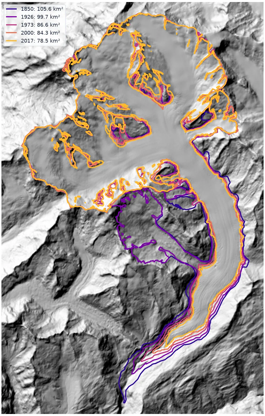
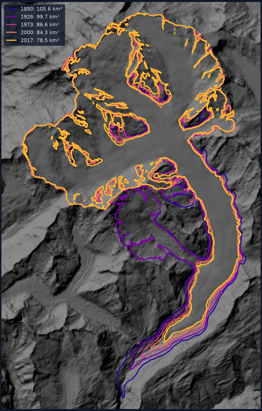
Dated outlines, an equal-area DEM, area per band
1. Get dated outlines
The Global Land Ice Measurements from Space (GLIMS) database holds outlines of the same glacier from different years and analysts, each tagged with its source date. A WFS request returns them as GeoJSON:
print(outlines[["year", "analyst", "km2"]].to_string(index=False)) year analyst km2
1850 University of Zurich-Irchel 105.616576
1926 GLAMOS (Glacier Monitoring Switzerland) 99.682794
1973 University of Zurich-Irchel 86.629190
1998 University of Zurich-Irchel 82.341352
2000 Friedrich-Alexander University (FAU) 84.278080
2003 University of Zurich-Irchel 82.625635
2003 University of Zurich-Irchel 81.790440
2008 University of Fribourg 78.130260
2009 University of Fribourg 78.131203
2011 Friedrich-Alexander University (FAU) 75.803935
2013 Friedrich-Alexander University (FAU) 79.539673
2015 University of Zurich-Irchel 77.324281
2017 GLAMOS (Glacier Monitoring Switzerland) 78.493588
The areas are not a smooth decline — some later outlines are larger than earlier ones, because different analysts drew boundaries differently, and because the glacier's identity changed: the Mittelaletsch, a tributary in 1850, has been inventoried as a separate glacier since at least 1973 (see glacier inventories explained). For hypsometry, pick outlines with a consistent definition, or say clearly that the comparison mixes them.
2. Put the DEM on an equal-area grid
Copernicus GLO-30 is delivered in degrees: at 46.4° N a cell is about 31 × 21 m, not square, and summing cell counts in degrees would mis-state areas. Reprojecting to the Swiss LV95 grid (EPSG:2056) at 25 m makes every cell 625 m²:
with rasterio.open("data/aletsch_dem_2056.tif") as src:
    print(src.crs.to_epsg(), src.res, src.shape, f"elevation {z[z > 100].min():.0f}-{z.max():.0f} m (edge cells outside the source tiles are 0)")
2056 (25.0, 25.0) (1164, 992) elevation 103-4144 m (edge cells outside the source tiles are 0)
3. Count area per band
The quick answer's histogram gives area per 100 m band. Comparing years shows where area was lost:
lost = h[1850] - h[2017]
for lo, hi in ((1400, 2500), (2500, 3000), (3000, 4300)):
    sel = (lost.index >= lo) & (lost.index < hi)
    print(f"{lo}-{hi} m: lost {lost[sel].sum():5.2f} km² of {h.loc[sel, 1850].sum():5.2f} ({lost[sel].sum() / h.loc[sel, 1850].sum():.0%})")
mittel = g[(g.glac_id == "G008010E46463N") & (g.line_type == "glac_bound")].to_crs(2056).sort_values("src_date")
gone = make_valid(outlines.loc[outlines.year == 1850, "geometry"].iloc[0]).difference(
       make_valid(outlines.loc[outlines.year == 2017, "geometry"].iloc[0]))
in_mittel = gone.intersection(make_valid(mittel.geometry.iloc[0]).buffer(200))
print(f"in the 1850 outline but not 2017: {gone.area / 1e6:.1f} km², of which {in_mittel.area / 1e6:.1f} km² is the "
      f"Mittelaletsch basin, inventoried separately from {mittel.src_date.iloc[0].year} ({mittel.area.iloc[0] / 1e6:.1f} km² then)")
1400-2500 m: lost 10.70 km² of 23.24 (46%)
2500-3000 m: lost 7.73 km² of 26.88 (29%)
3000-4300 m: lost 8.71 km² of 55.49 (16%)
in the 1850 outline but not 2017: 27.5 km², of which 9.5 km² is the Mittelaletsch basin, inventoried separately from 1973 (8.3 km² then)
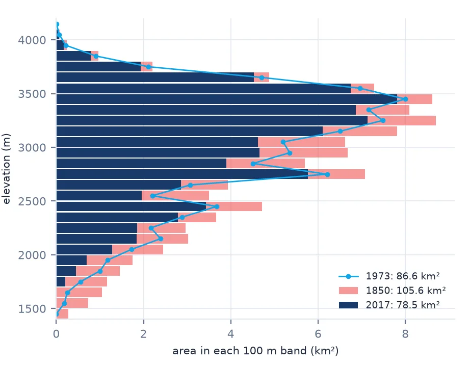
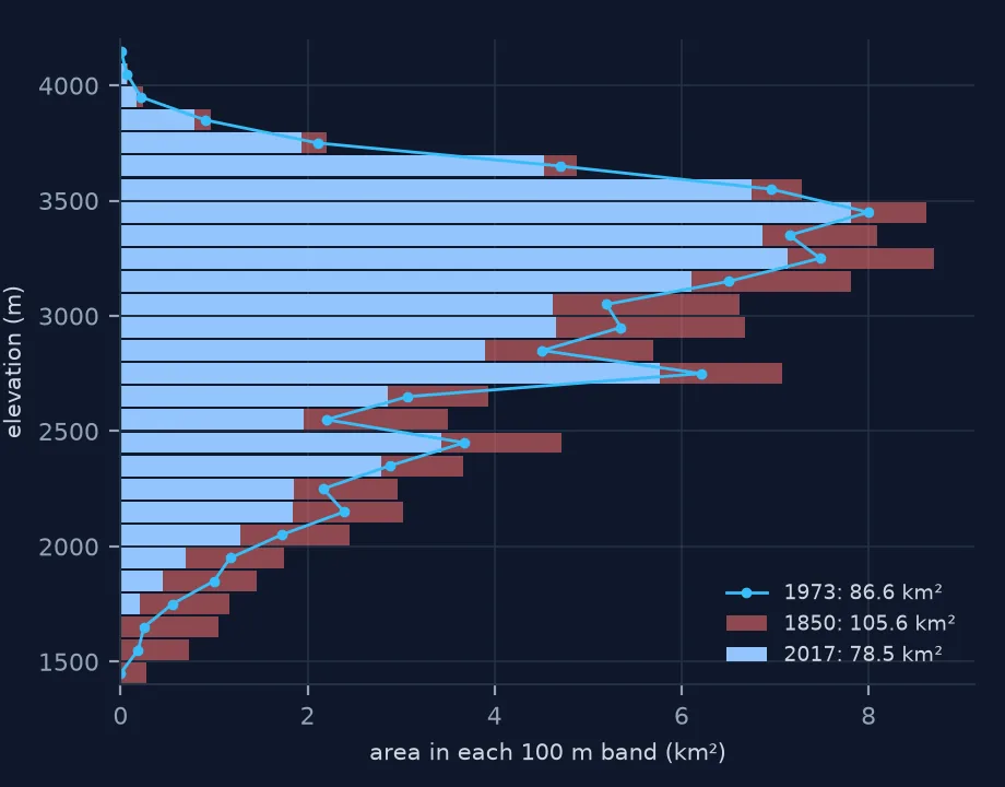
Proportionally the loss is concentrated low down: the bands below 2,500 m lost almost half of their 1850 area, those above 3,000 m a sixth. In absolute terms the higher bands contribute too — but a third of all the "lost" area, 9.5 km², is the Mittelaletsch basin, which in 1850 flowed into the Great Aletsch and was counted as part of it, and by 1973 was mapped as a glacier of its own. That ice did not melt between the two outlines; it changed name.
4. Remember the DEM's date
The DEM records the surface around 2011–2015. Inside the 1850 outline it gives today's elevations, not 1850's — and the tongue has thinned by hundreds of metres since. So the 1850 hypsometry here is "the terrain the 1850 glacier covered, at today's height", which is right for asking where the glacier was and wrong for asking how high its surface stood. The ground inside the 1850 outline but outside the 2017 one shows both effects — the deglaciated tongue low down, and the definitional differences up high:
tongue = outlines.loc[outlines.year == 1850, "geometry"].iloc[0].difference(outlines.loc[outlines.year == 2017, "geometry"].iloc[0])
inside = rasterize([(tongue, 1)], out_shape=z.shape, transform=tr, dtype="uint8").astype(bool)
low = inside & (z < 2500)
print(f"inside 1850 but not 2017: {inside.sum() * res * res / 1e6:.1f} km² (median today {np.median(z[inside]):.0f} m); "
      f"below 2,500 m: {low.sum() * res * res / 1e6:.1f} km², median today {np.median(z[low]):.0f} m")
inside 1850 but not 2017: 27.5 km² (median today 2739 m); below 2,500 m: 10.7 km², median today 2025 m
5. Summarise the shape
Two numbers summarise hypsometry: the median elevation, which tracks the balance between high and low area, and the area–altitude distribution's skew. The median of the Aletsch area has risen by about 100 m since 1850 as the low tongue disappeared.
Hypsometry for every GLIMS outline
The data used on this page
Glacier outlines from the GLIMS Glacier Database (NSIDC), glacier G008032E46504N (Grosser Aletschgletscher), records by the University of Zurich (1850, 1973) and GLAMOS — Glacier Monitoring Switzerland (2017). Elevation: Copernicus DEM GLO-30 (© DLR e.V. 2010–2014 and © Airbus Defence and Space GmbH 2014–2018, provided under COPERNICUS by the European Union and ESA) from the AWS Open Data registry.
from pathlib import Path

import geopandas as gpd
import numpy as np
import pandas as pd
import rasterio
import requests
from rasterio.features import rasterize
from rasterio.merge import merge
from rasterio.warp import Resampling, calculate_default_transform, reproject
from shapely import make_valid

Path("data").mkdir(exist_ok=True)
GLIMS = ("https://www.glims.org/geoserver/GLIMS/ows?service=WFS&version=1.0.0&request=GetFeature"
         "&typeName=GLIMS:GLIMS_Glacier_Outlines&outputFormat=application/json&bbox=7.95,46.40,8.15,46.56")
if not Path("data/glims_aletsch.json").exists():
    Path("data/glims_aletsch.json").write_bytes(requests.get(GLIMS, timeout=300).content)
g = gpd.read_file("data/glims_aletsch.json")
outlines = g[(g.glac_id == "G008032E46504N") & (g.line_type == "glac_bound")].to_crs(2056)
outlines = outlines[outlines.area > 1e6].sort_values("src_date").drop_duplicates("src_date", keep="last")
outlines = outlines.assign(year=outlines.src_date.dt.year, km2=outlines.area / 1e6, analyst=outlines.chief_affl)

if not Path("data/aletsch_dem_2056.tif").exists():
    COP = "https://copernicus-dem-30m.s3.amazonaws.com/Copernicus_DSM_COG_10_{t}_DEM/Copernicus_DSM_COG_10_{t}_DEM.tif"
    srcs = [rasterio.open(COP.format(t=t)) for t in ("N46_00_E007_00", "N46_00_E008_00")]
    mos, mtr = merge(srcs, bounds=(7.88, 46.33, 8.2, 46.59))
    t, w, h = calculate_default_transform(srcs[0].crs, "EPSG:2056", mos.shape[2], mos.shape[1],
                                          7.88, 46.33, 8.2, 46.59, resolution=25)
    out = np.zeros((h, w), np.float32)
    reproject(mos[0], out, src_transform=mtr, src_crs=srcs[0].crs, dst_transform=t, dst_crs="EPSG:2056",
              resampling=Resampling.bilinear)
    with rasterio.open("data/aletsch_dem_2056.tif", "w", driver="GTiff", height=h, width=w, count=1, dtype="float32",
                       crs="EPSG:2056", transform=t, compress="deflate") as dst:
        dst.write(out, 1)
print(len(outlines), "dated outlines;", Path("data/aletsch_dem_2056.tif").stat().st_size // 1_000_000, "MB DEM")
13 dated outlines; 3 MB DEM
Example 1: hypsometry for every outline
rows = []
for _, r in outlines.iterrows():
    m = rasterize([(r.geometry, 1)], out_shape=z.shape, transform=tr, dtype="uint8").astype(bool)
    rows.append({"date": r.src_date.date(), "km2": round(r.km2, 1), "lowest point (m)": int(z[m].min()),
                 "median (m)": int(np.median(z[m])), "share below 2500 m": f"{(z[m] < 2500).mean():.0%}"})
print(pd.DataFrame(rows).to_string(index=False))
date km2 lowest point (m) median (m) share below 2500 m
1850-09-01 105.6 1408 3042 22%
1926-09-01 99.7 1492 3077 20%
1973-09-01 86.6 1528 3113 18%
1998-08-31 82.3 1563 3158 16%
2000-08-20 84.3 1563 3153 16%
2003-08-06 82.6 1564 3155 16%
2003-08-13 81.8 1564 3152 16%
2008-09-30 78.1 1628 3149 16%
2009-09-15 78.1 1628 3149 16%
2011-09-13 75.8 1681 3179 14%
2013-08-01 79.5 1728 3154 16%
2015-08-29 77.3 1681 3162 15%
2017-09-01 78.5 1681 3149 16%
The lowest point rises steadily — the terminus retreating up its valley — while the median and the share of area below 2,500 m move less regularly, because the outlines differ in which tributaries and fragments they include.
Example 2: the area–altitude curve
The cumulative distribution, normalised, compares shapes independent of size:
for y in (1850, 2017):
    c = h[y].cumsum() / h[y].sum()
    q = {p: int(c.index[np.searchsorted(c.values, p)]) for p in (0.1, 0.5, 0.9)}
    print(y, "10th, 50th, 90th percentile elevation of area:", q)
1850 10th, 50th, 90th percentile elevation of area: {0.1: 2100, 0.5: 3000, 0.9: 3500}
2017 10th, 50th, 90th percentile elevation of area: {0.1: 2300, 0.5: 3100, 0.9: 3500}
Two datasets, two moments
Hypsometry joins two datasets that describe different moments: an outline, which says where the glacier was on a date, and a DEM, which says how high the ground was when it was measured. When the two are close in time — a 2015 outline over a 2013 DEM — the result is the glacier's true area–altitude distribution. When they are far apart, as with 1850 over 2013, it is the distribution of the glacier's footprint over today's terrain.
That distinction matters because glaciers thin as well as shrink. The Aletsch tongue that reached 1,400 m today's ground level in 1850 stood far higher then; the 1850 bands below 2,000 m here are lower than the ice surface ever was. Questions about where area was lost are answered well; questions about how high the glacier reached need a DEM of the right date or a reconstruction.
The area numbers themselves carry a second caveat. A glacier inventory decides what counts as one glacier, and that decision changes: the Mittelaletsch was part of the Great Aletsch in the 1850 reconstruction and a separate entry from 1973, and different analysts draw tributary boundaries and fragments differently in years only two apart. The low-elevation loss, where the tongue retreated, is robust to that; much of the high-elevation difference is a change of identity rather than of ice.
Debris-covered ice and small polygons
- Reproject the DEM to a metric equal-area grid before counting area.
- Use outlines with one definition for a time series, or say that they are mixed.
- The DEM's date sets what the elevations mean; old outlines over a new DEM give footprints, not surfaces.
- Debris-covered ice is part of the glacier; GLIMS marks it separately (
debris_cov). - Small polygons in a record are nunataks or fragments; keep the main outline or handle them explicitly.
- Band width of 50–100 m suits a 30 m DEM; narrower bands are noisy.
Internal links
- Glacier inventories explained — why the outlines disagree
- How to measure glacier retreat — the terminus over time
- How to find the snow line elevation — the other half of a glacier's balance
- How to analyse snow depth from GHCN-Daily — station snow records
- How to measure change from an old map — the same caution with dates and definitions
FAQ
What is glacier hypsometry?
The distribution of a glacier's area with elevation, usually as area per elevation band. It controls how sensitive the glacier is to changes in the snow line.
How do I calculate glacier hypsometry in Python?
Reproject a DEM to an equal-area grid, rasterise the glacier outline onto it with rasterio.features.rasterize, and histogram the DEM values inside the outline.
Where did the Great Aletsch Glacier lose area since 1850?
Proportionally from its tongue: the bands below 2,500 m lost 46% of their 1850 area by 2017, those above 3,000 m 16%. A third of the total difference is the Mittelaletsch, a tributary in 1850 that has been inventoried as a separate glacier since 1973.
Can I use a modern DEM with an old glacier outline?
For where the glacier was, yes. For how high its surface stood, no — the glacier has thinned, so the modern DEM is lower than the old ice surface.