How to Map Sea Surface Temperature Trends in Python

Problem statement

How fast is the ocean warming, and where? A trend map answers both: one number per grid cell, the slope of a line through decades of temperatures. Getting it right takes complete years so the seasonal cycle does not leak into the slope, a vectorised fit so thousands of cells do not need a loop, a way to say which trends stand out from year-to-year noise, and area weighting for any global summary.

This page fits linear trends to annual mean ERSST v5 sea surface temperatures for every 2° cell from 1982 to 2025, maps them, summarises the global ocean, tests which cells have trends well beyond their noise, and compares the recent period with the longer record since 1950.

Quick answer

Average each complete year, then fit all cells at once with numpy.polyfit, which accepts a 2-D array of series:

ann = SST.sel(time=slice("1982", "2025")).groupby("time.year").mean()
years = ann.year.values
Y = ann.values.reshape(len(years), -1)
ok = np.isfinite(Y).all(axis=0)
slope = np.full(Y.shape[1], np.nan)
slope[ok] = np.polyfit(years, Y[:, ok], 1)[0] * 10                              # °C per decade
trend = xr.DataArray(slope.reshape(ann.shape[1:]), coords={"latitude": ann.latitude, "longitude": ann.longitude})
w = np.cos(np.deg2rad(trend.latitude))
print(f"cells fitted: {int(ok.sum()):,}; area-weighted mean trend 1982-2025: {float(trend.weighted(w).mean()):+.3f} °C per decade")
print(f"warming cells: {float((w * (trend > 0)).sum() / (w * trend.notnull()).sum()):.0%} of the ocean area")

cells fitted: 10,972; area-weighted mean trend 1982-2025: +0.135 °C per decade
warming cells: 85% of the ocean area

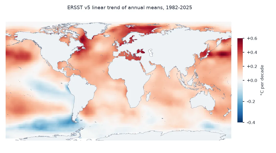
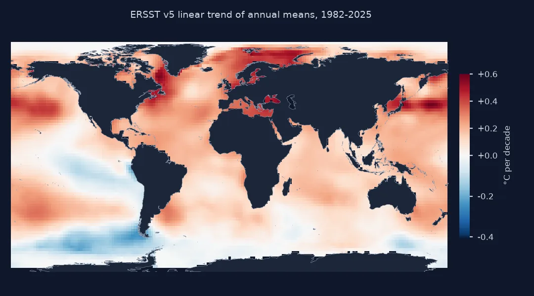
Fitted to annual means from 1982 to 2025, the 10,972 ocean cells warmed by 0.135 °C per decade on average, weighted by area, and 85% of the ocean area warmed.

Complete years, fastest warming, trends beyond the noise

1. Complete years only

A partial year has the wrong share of winter and summer. Check the months in each year before averaging:

months = SST.time.dt.year.to_series().value_counts().sort_index()
print(f"years {months.index.min()}-{months.index.max()}; incomplete: {months[months < 12].to_dict()}")
print(f"annual mean array: {ann.sizes['year']} years x {ann.sizes['latitude']} x {ann.sizes['longitude']} cells")

years 1950-2026; incomplete: {2026: 8}
annual mean array: 44 years x 89 x 180 cells

2026 has only eight months in the file, so the fit stops at 2025: 44 complete years.

2. Where it is warming fastest, and the exceptions

List the fastest-warming and fastest-cooling cells, and the latitude bands:

t = trend.to_series().dropna()
print("fastest warming:", ", ".join(f"{la:.0f}°, {lo:.0f}°: {v:+.2f}" for (la, lo), v in t.nlargest(3).items()))
print("cooling:", ", ".join(f"{la:.0f}°, {lo:.0f}°: {v:+.2f}" for (la, lo), v in t.nsmallest(3).items()))
for a, b in ((-90, -60), (-60, -30), (-30, 0), (0, 30), (30, 60), (60, 90)):
    band = trend.sel(latitude=slice(a, b))
    print(f"{a:>4} to {b:>3}: {float(band.weighted(np.cos(np.deg2rad(band.latitude))).mean()):+.3f} °C per decade")

fastest warming: 66°, -86°: +0.63, 40°, 166°: +0.59, 66°, -84°: +0.59
cooling: -54°, -72°: -0.25, -52°, -70°: -0.25, -54°, -70°: -0.25
 -90 to -60: -0.037 °C per decade
 -60 to -30: +0.086 °C per decade
 -30 to   0: +0.108 °C per decade
   0 to  30: +0.152 °C per decade
  30 to  60: +0.286 °C per decade
  60 to  90: +0.220 °C per decade

The fastest-warming cells are in Hudson Bay, ice-covered for much of the year, and in the Kuroshio Extension east of Japan, at up to 0.63 °C per decade. The cooling cells, at -0.25 °C per decade, are in the Southern Ocean south of Chile. By latitude, warming is fastest between 30°N and 60°N, 0.286 °C per decade, and the band south of 60°S cooled slightly.

3. Which trends stand out from the noise

Compare each slope with its standard error from the residuals; a ratio above 2 is roughly a 95% test, ignoring autocorrelation:

fit = np.polyfit(years, Y[:, ok], 1)
resid = Y[:, ok] - (np.outer(years, fit[0]) + fit[1])
se = np.sqrt((resid ** 2).sum(0) / (len(years) - 2) / ((years - years.mean()) ** 2).sum()) * 10
ratio = np.abs(slope[ok]) / se
wk = np.cos(np.deg2rad(np.repeat(ann.latitude.values, ann.sizes["longitude"])))[ok]
print(f"cells with |trend| > 2 standard errors: {(ratio > 2).mean():.0%}; by area {(wk * (ratio > 2)).sum() / wk.sum():.0%}")
print(f"median standard error {np.median(se):.3f} °C per decade")

cells with |trend| > 2 standard errors: 74%; by area 76%
median standard error 0.034 °C per decade

Three quarters of cells, 76% of the area, have a trend more than twice its standard error; the typical standard error is 0.034 °C per decade. With autocorrelation the real share would be smaller.

Since 1982 and since 1950

The data used on this page

Monthly NOAA ERSST v5 on its 2° grid from January 1950 to August 2026, from NOAA CoastWatch's ERDDAP. ERSST reconstructs sea surface temperature from ship, buoy and float observations; it does not use satellites. The grid also covers the Caspian Sea, a lake, which the setup masks.

from pathlib import Path

import numpy as np
import pandas as pd
import requests
import xarray as xr

Path("data").mkdir(exist_ok=True)
p = Path("data/ersst_global_1950_202608.nc")
if not p.exists():
    q = "sst[(1950-01-01):1:(2026-08-01)][(0.0)][(-88):1:(88)][(-180):1:(178)]"
    p.write_bytes(requests.get(f"https://coastwatch.pfeg.noaa.gov/erddap/griddap/nceiErsstv5_LonPM180.nc?{q}", timeout=900).content)
SST = xr.open_dataset(p).sst.squeeze(drop=True)
caspian = (SST.latitude > 35) & (SST.latitude < 48) & (SST.longitude > 45) & (SST.longitude < 56)
print(f"Caspian Sea cells in the grid: {int(SST.isel(time=-1).where(caspian).notnull().sum())} (a lake: masked)")
SST = SST.where(~caspian)
print(f"{SST.sizes['time']} months, {SST.sizes['latitude']} x {SST.sizes['longitude']} cells; file {p.stat().st_size / 1e6:.0f} MB")

Caspian Sea cells in the grid: 16 (a lake: masked)
920 months, 89 x 180 cells; file 59 MB

The ERSST grid has 16 cells over the Caspian Sea, which the setup masks; left in, they top the list of fastest-warming cells. The file holds 920 months on 89 by 180 cells.

Example 1: since 1982 and since 1950

Fit the same way over 1950–2025 and compare the global mean and the share of cells warming:

def fit_trend(a, b):
    an = SST.sel(time=slice(a, b)).groupby("time.year").mean()
    Yb = an.values.reshape(an.sizes["year"], -1); okb = np.isfinite(Yb).all(0)
    s = np.full(Yb.shape[1], np.nan); s[okb] = np.polyfit(an.year.values, Yb[:, okb], 1)[0] * 10
    tr = xr.DataArray(s.reshape(an.shape[1:]), coords={"latitude": an.latitude, "longitude": an.longitude})
    wb = np.cos(np.deg2rad(tr.latitude))
    return float(tr.weighted(wb).mean()), float((wb * (tr > 0)).sum() / (wb * tr.notnull()).sum())
for a, b in (("1950", "2025"), ("1982", "2025"), ("2000", "2025")):
    m, sh = fit_trend(a, b)
    print(f"{a}-{b}: mean {m:+.3f} °C per decade, warming area {sh:.0%}")

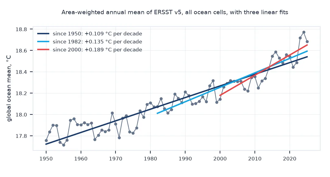
1950-2025: mean +0.109 °C per decade, warming area 98%
1982-2025: mean +0.135 °C per decade, warming area 85%
2000-2025: mean +0.189 °C per decade, warming area 92%

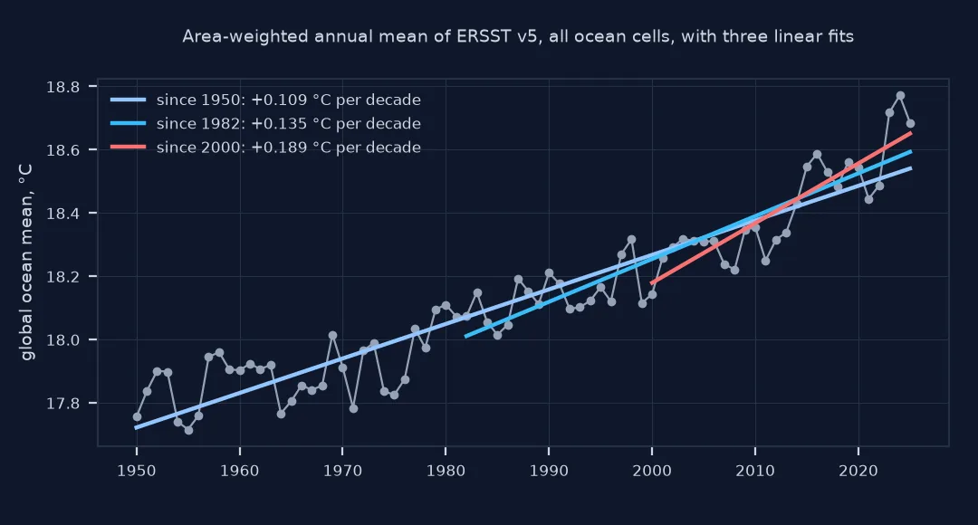
The longer the period, the slower the average warming: 0.109 °C per decade since 1950, 0.135 since 1982, 0.189 since 2000. Since 1950, 98% of the ocean area has warmed.

A linear trend as the simplest summary

A linear trend is the simplest summary of change over time, and over a few decades of a warming climate it fits reasonably well, though warming has accelerated and a single slope smooths that. Fitting annual means rather than months removes the seasonal cycle without needing a climatology, and fitting every cell with one call to polyfit on a two-dimensional array is how a global map of trends takes a second rather than minutes. The global summary must weight cells by area, because a 2° cell at 60° latitude covers half the ocean of one at the equator.

The standard error test treats each year as independent, which ocean temperatures are not: a warm year tends to follow a warm year, so the effective number of independent years is smaller and real uncertainties are larger than this test assumes. For a map, the ratio is still a useful screen of where a trend is large relative to year-to-year variability. The exceptions on the map are as informative as the rule: south of 60°S the mean trend since 1982 is slightly negative, and the strongest cooling cells lie in the Southern Ocean off southern Chile, while the fastest warming is in the northern mid- and high latitudes, including the Kuroshio Extension off Japan.

Sea ice, period sensitivity and non-linear change

• Sea ice: cells under seasonal ice hold values near the freezing point for months, which damps their trends; mask cells with ice for part of the year if that matters.
• Period sensitivity: trends over a few decades depend on where they start and end, especially with El Niño years at the ends; report the period.
• ERSST at high latitudes: observations are sparse in the Southern Ocean before the Argo era, and the reconstruction relies more on statistics there.
• Non-linear change: for acceleration, fit separate periods, a quadratic, or a smooth curve instead of one line.

Internal links

• How to compute the global mean sea surface temperature in Python — the area-weighted series behind the mean trend
• Fixing global SST means that ignore cell area — why the weights matter
• Sea surface temperature explained — ERSST and OISST compared

FAQ

How do I calculate a trend for every grid cell in Python?

Reshape the data to years by cells and pass it to numpy.polyfit(years, Y, 1), which fits all columns at once; the first row of the result is the slope.

How fast is the ocean warming?

On this page, the area-weighted mean trend of ERSST annual means from 1982 to 2025 is printed in the quick answer, in °C per decade.

Why use annual means for trends?

They remove the seasonal cycle and reduce noise; monthly data need anomalies first, or the seasonal cycle biases the fit at the ends.

Is a trend significant if it is twice its standard error?

Roughly, for independent data; because ocean temperatures are autocorrelated, real uncertainty is larger, so treat the test as a screen.