How to Compute the Global Mean Sea Surface Temperature in Python

On this page

Problem statement

The global mean sea surface temperature is one of the headline numbers of climate monitoring, and 2023 and 2024 broke its records month after month. Computing it from a gridded product looks like a one-line mean, but the number depends on three choices: which latitudes count as the global ocean, how cells of different sizes are weighted, and whether the result is reported as a temperature or as an anomaly from a base period. Different choices give different headlines from the same data.

This page computes the monthly global mean from ERSST v5 since 1950, for 60°S–60°N with area weights, turns it into anomalies against 1991–2020, finds the record months and years, and compares the 60°S–60°N mean with one over every ocean cell.

Quick answer

Select the latitudes, weight each cell by the cosine of its latitude, and average over space for each month:

band = SST.sel(latitude=slice(-60, 60))
gm = band.weighted(np.cos(np.deg2rad(band.latitude))).mean(["latitude", "longitude"]).to_series()
clim = gm["1991":"2020"].groupby(gm["1991":"2020"].index.month).mean()
anom = gm - gm.index.month.map(clim).values
print(f"{gm.index[0]:%b %Y} to {gm.index[-1]:%b %Y}; latest {anom.index[-1]:%b %Y}: {gm.iloc[-1]:.2f} °C, anomaly {anom.iloc[-1]:+.2f} °C")
print(f"warmest anomaly: {anom.max():+.2f} °C in {anom.idxmax():%B %Y}")

Jan 1950 to Aug 2026; latest Aug 2026: 21.08 °C, anomaly +0.67 °C
warmest anomaly: +0.67 °C in August 2026

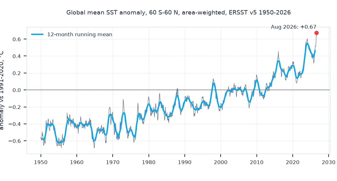
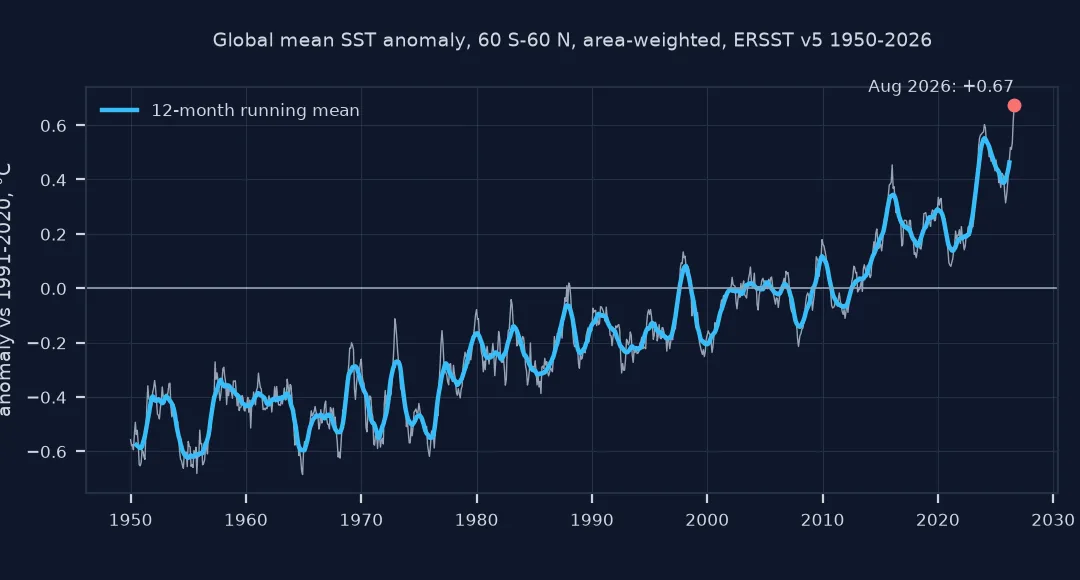
The series runs from January 1950 to August 2026. The latest month is also the warmest relative to normal: August 2026, 21.08 °C, 0.67 °C above the 1991–2020 August mean.

Chart of the monthly global mean sea surface temperature anomaly for 60 south to 60 north against 1991 to 2020, from about minus 0.5 degrees in the 1950s to the record of plus 0.67 in August 2026, with a 12-month running mean that rises steeply after 2022. — Global mean SST anomaly.

The band and its weights, record months and years

1. The band and the weights

Polar seas are partly ice-covered and their temperatures are pinned near freezing, so many monitoring series use 60°S–60°N. Within the band, cells near the equator are larger than those near 60°:

cells = band.notnull().isel(time=-1)
w = np.cos(np.deg2rad(band.latitude))
print(f"ocean cells in 60S-60N: {int(cells.sum()):,}; weight at the equator 1.00, at 60° {float(np.cos(np.deg2rad(60))):.2f}")
print(f"cells between 50° and 60° in either hemisphere: {int(cells.sel(latitude=abs(cells.latitude) >= 50).sum()):,} "
      f"({float(cells.sel(latitude=abs(cells.latitude) >= 50).sum() / cells.sum()):.0%} of cells, "
      f"{float((cells * w).sel(latitude=abs(cells.latitude) >= 50).sum() / (cells * w).sum()):.0%} of area)")

ocean cells in 60S-60N: 8,281; weight at the equator 1.00, at 60° 0.50
cells between 50° and 60° in either hemisphere: 1,581 (19% of cells, 13% of area)

Between 60°S and 60°N there are 8,281 ocean cells. The 1,581 between 50° and 60° are 19% of the cells but 13% of the area, because a cell at 60° has half the weight of one at the equator.

2. Record months

Rank the anomalies and list the warmest months and when each record was set:

top = anom.nlargest(6)
print(top.round(2).rename(lambda t: t.strftime("%b %Y")).to_string())
records = anom[anom == anom.cummax()]
print(f"months that set a new all-time record since 2000: {(records.index.year >= 2000).sum()}, the last in {records.index[-1]:%B %Y}")

time
Aug 2026    0.67
Jul 2026    0.62
Jan 2024    0.60
Feb 2024    0.59
Dec 2023    0.57
Nov 2023    0.57
months that set a new all-time record since 2000: 19, the last in August 2026

The six warmest months are July and August 2026 and four months from November 2023 to February 2024. Nineteen months since 2000 have set a new all-time record, the latest in August 2026, during the El Niño that the index guide follows.

From a grid to one number.

3. Record years

Average complete years and rank them:

yr = anom.groupby(anom.index.year).agg(["mean", "size"])
yr = yr[yr["size"] == 12]["mean"]
print(yr.nlargest(5).round(3).to_string())
print(f"1950s mean anomaly {yr.loc[1950:1959].mean():+.2f} °C; 2015-2024 {yr.loc[2015:2024].mean():+.2f} °C")

time
2024    0.508
2023    0.448
2025    0.396
2016    0.284
2015    0.267
1950s mean anomaly -0.48 °C; 2015-2024 +0.28 °C

2024 is the warmest complete year, 0.508 °C above the 1991–2020 mean, ahead of 2023 and 2025; 2016 and 2015, the previous El Niño years, are fourth and fifth. The 1950s averaged 0.48 °C below the 1991–2020 normal, the decade 2015–2024 0.28 °C above it.

Sixty south to sixty north against every cell

The data used on this page

Monthly NOAA ERSST v5 on its 2° grid from January 1950 to August 2026, from NOAA CoastWatch's ERDDAP.

from pathlib import Path

import numpy as np
import pandas as pd
import requests
import xarray as xr

Path("data").mkdir(exist_ok=True)
p = Path("data/ersst_global_1950_202608.nc")
if not p.exists():
    q = "sst[(1950-01-01):1:(2026-08-01)][(0.0)][(-88):1:(88)][(-180):1:(178)]"
    p.write_bytes(requests.get(f"https://coastwatch.pfeg.noaa.gov/erddap/griddap/nceiErsstv5_LonPM180.nc?{q}", timeout=900).content)
SST = xr.open_dataset(p).sst.squeeze(drop=True)
print(f"{SST.sizes['time']} months from {pd.Timestamp(SST.time.values[0]):%b %Y} to {pd.Timestamp(SST.time.values[-1]):%b %Y}")

920 months from Jan 1950 to Aug 2026

The file holds 920 months.

Example 1: 60°S–60°N against every ocean cell

Include the polar seas and compare the two series:

allo = SST.weighted(np.cos(np.deg2rad(SST.latitude))).mean(["latitude", "longitude"]).to_series()
a2 = allo - allo.index.month.map(allo["1991":"2020"].groupby(allo["1991":"2020"].index.month).mean()).values
print(f"mean temperature, 1991-2020: 60S-60N {gm['1991':'2020'].mean():.2f} °C, all ocean {allo['1991':'2020'].mean():.2f} °C")
print(f"anomaly in {anom.idxmax():%b %Y}: 60S-60N {anom.max():+.2f} °C, all ocean {a2[anom.idxmax()]:+.2f} °C")
print(f"trend 1982-2025: 60S-60N {np.polyfit(np.arange(528), anom['1982':'2025'].values, 1)[0] * 120:+.3f}, all ocean {np.polyfit(np.arange(528), a2['1982':'2025'].values, 1)[0] * 120:+.3f} °C per decade")

mean temperature, 1991-2020: 60S-60N 20.28 °C, all ocean 18.30 °C
anomaly in Aug 2026: 60S-60N +0.67 °C, all ocean +0.65 °C
trend 1982-2025: 60S-60N +0.142, all ocean +0.136 °C per decade

Including the polar seas lowers the mean temperature by about 2 °C, to 18.30 °C, because of the near-freezing ice-covered cells, but changes the anomalies and the trend only slightly: +0.65 against +0.67 °C in August 2026, and 0.136 against 0.142 °C per decade.

The warmest years.

Why a global mean needs weights

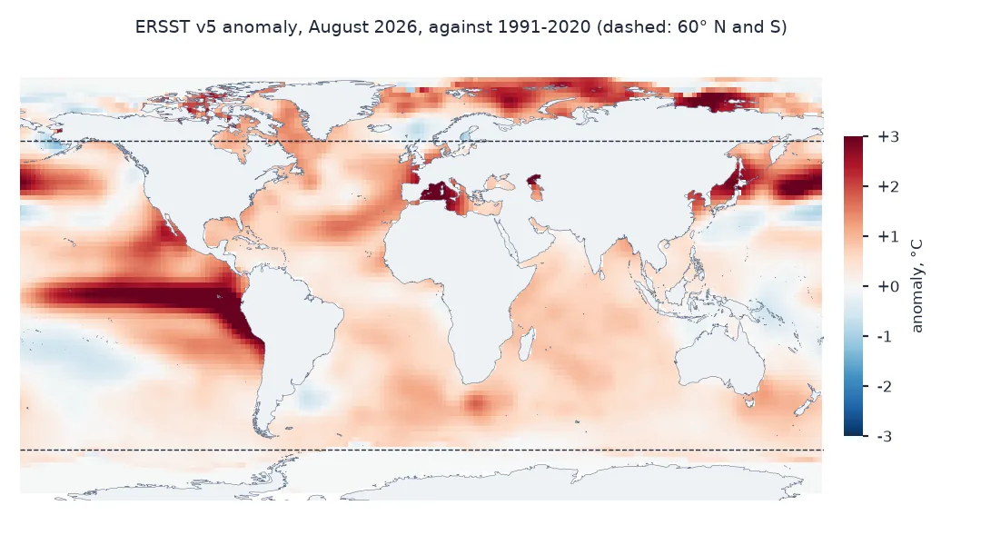
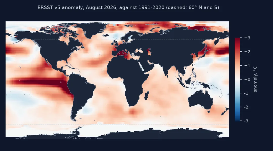
World map of the ERSST anomaly for August 2026 against 1991 to 2020: a strong warm tongue along the equatorial Pacific off South America from El Niño, warm water across the North Pacific off Japan, the Mediterranean and Arctic seas, and small cool patches in the Southern Ocean; dashed lines mark 60 north and south. — The record month.

A global mean from a latitude-longitude grid needs weights because cells are not equal: a 2° cell at 60° covers half the area of one at the equator, and an unweighted mean would count the high-latitude oceans twice over. The cosine of the cell's central latitude is the standard weight for a regular grid; land cells are already missing, so the mean is over ocean only. The band matters for a different reason: in the polar seas, sea ice holds the surface near -1.8 °C and the reconstructions rely heavily on ice concentration, so many monitoring series leave them out.

Anomalies, not temperatures, are what records are about. The global mean temperature has a seasonal cycle, from the different land-ocean distribution of the two hemispheres, so a March and a September are not comparable directly; subtracting each month's 1991–2020 mean removes it. Records in 2023 and 2024 were set by margins that are large relative to the series' month-to-month noise, which is why they drew so much attention. Other products, OISST or the ERA5 reanalysis, give slightly different values because of different inputs and methods, but the same ranking of recent years.

Preliminary months, base periods and lakes

Before quoting a global mean.

Preliminary months: the latest ERSST month is updated when more observations arrive; recent records can change by a few hundredths.
Base period: anomalies against 1991–2020 are smaller than against 1951–1980 or 1971–2000 by the warming between them.
Different bands: some products report 60°S–60°N, others the whole ice-free ocean; check before comparing numbers.
Lakes in the grid: ERSST's grid includes 16 cells over the Caspian Sea, a lake, inside 60°S–60°N; a tiny share of the area, but mask them for an ocean-only figure.
Weights on other grids: on irregular or projected grids, use each cell's actual area instead of the cosine of latitude.

Internal links

How to map sea surface temperature trends in Python — the same data cell by cell
Fixing global SST means that ignore cell area — what happens without weights
How to compute an El Niño index from sea surface temperature in Python — the tropical Pacific part of the story

FAQ

How do I calculate the global mean sea surface temperature in Python?

Select 60°S–60°N, weight each cell by the cosine of its latitude with xarray's weighted, and average over latitude and longitude for each month.

Why is the global SST average limited to 60°S-60°N?

Polar seas are partly covered by ice, where surface temperatures are held near freezing and are estimated from ice concentration rather than measured, so many series exclude them.

What was the warmest month for global sea surface temperature?

In ERSST v5 as downloaded for this page, the warmest anomaly and its month are printed in the quick answer.

Why use anomalies instead of temperatures?

The global mean has a seasonal cycle; anomalies against each month's base-period mean make months comparable.