How to Test for Near-Repeat Burglary in Python

Problem statement

After a burglary, the risk of another one nearby rises for a while: the same burglar returns to a place they know, or a neighbouring house with the same layout. This near-repeat pattern is one of the best-replicated findings in crime analysis, and the basis of warning neighbours after a break-in. Whether it holds in a given city, over what distance and for how long, is an empirical question with a standard test: the Knox test, which counts pairs of incidents close in both space and time and compares the count with what shuffling the dates would give.

This page runs a Knox test on Chicago's 2024 burglaries with SciPy, measures how much more often pairs fall close in space and time than chance, separates repeats at the same location from near repeats, and checks how much of the result comes from incidents recorded at the same moment.

Quick answer

Find every pair within the largest distance band with a KD tree, tabulate pairs by distance and time apart, and compare with tables built from shuffled dates:

i, j = cKDTree(XY).query_pairs(2400, output_type="ndarray").T
dist = np.hypot(*(XY[i] - XY[j]).T)

def knox(days):
    return np.histogram2d(dist, np.abs(days[i] - days[j]), bins=[D_BINS, T_BINS])[0]

obs = knox(DAYS)
sims = np.array([knox(RNG.permutation(DAYS)) for _ in range(999)])
ratio = pd.DataFrame(obs / sims.mean(axis=0), index=D_LABELS, columns=T_LABELS)
p = pd.DataFrame(((sims >= obs).sum(axis=0) + 1) / 1000, index=D_LABELS, columns=T_LABELS)
print(f"{len(XY):,} burglaries, {len(i):,} pairs within 2,400 ft")
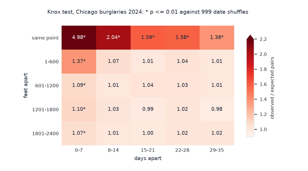
print("observed / expected pairs:"); print(ratio.round(2).to_string())

8,397 burglaries, 183,893 pairs within 2,400 ft
observed / expected pairs:
             0-7  8-14  15-21  22-28  29-35
same point  4.98  2.04   1.59   1.58   1.38
1-600       1.37  1.07   1.01   1.04   1.01
601-1200    1.09  1.01   1.04   1.03   1.01
1201-1800   1.10  1.03   0.99   1.02   0.98
1801-2400   1.07  1.01   1.00   1.02   1.02

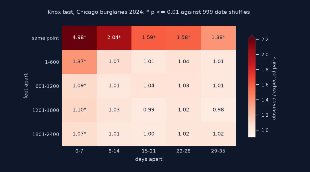
Pairs at the same point within a week are 4.98 times as common as chance, and still 1.38 times as common a month later. Within 600 feet, the first week has 1.37 times the expected pairs, and the second week 1.07. Beyond that the first-week ratio stays a little above one, 1.07 to 1.10, to the edge of the table.

Choose bands, read significance, check for duplicates

1. Choose the bands

The table needs distance and time bands. Distance in feet suits Chicago's grid, eight blocks to the mile, and Chicago publishes locations at block level, so the first band is the same point: repeats at one address or block. Time bands of a week are usual:

print("distance bands (ft):", D_LABELS)
print("time bands (days):", T_LABELS)
same_point = dist < 0.5
print(f"pairs at the same point: {same_point.sum():,}; burglaries sharing a point with another: {len(np.unique(np.r_[i[same_point], j[same_point]])):,}")

distance bands (ft): ['same point', '1-600', '601-1200', '1201-1800', '1801-2400']
time bands (days): ['0-7', '8-14', '15-21', '22-28', '29-35']
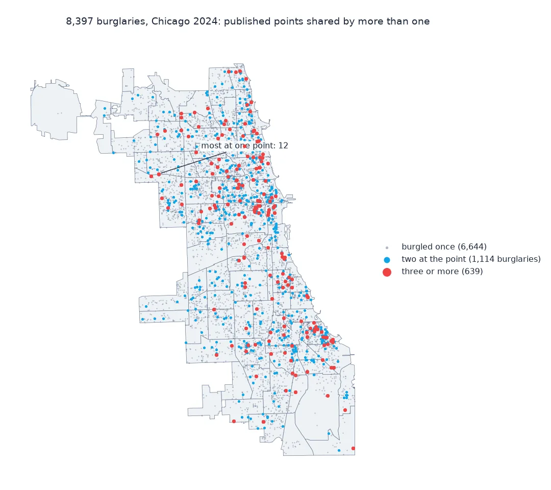
pairs at the same point: 1,573; burglaries sharing a point with another: 1,753

1,753 of the 8,397 burglaries, about one in five, share their published location with at least one other burglary that year.

2. Read the significance

Each cell's p-value is the share of the 999 shuffled tables with at least as many pairs as observed. With 999 shuffles the smallest possible value is 0.001:

print(p.to_string())
print(f"cells with p <= 0.01: {(p <= 0.01).values.sum()} of {p.size}")

              0-7   8-14  15-21  22-28  29-35
same point  0.001  0.001  0.001  0.001  0.003
1-600       0.001  0.043  0.381  0.158  0.391
601-1200    0.001  0.406  0.072  0.109  0.365
1201-1800   0.001  0.095  0.664  0.161  0.851
1801-2400   0.001  0.290  0.539  0.103  0.146
cells with p <= 0.01: 9 of 25

Every first-week cell is significant at 0.001, and so is the whole same-point row. Elsewhere, only the 1-600 ft second-week cell comes close, at 0.043, which a table of 25 cells can produce by chance. The faint first-week excess at 1,200-2,400 feet is weak but consistent: hundreds of extra pairs among thousands.

3. Check for duplicates of one event

A burglary of several flats in one building, or an incident split into several records, gives pairs at the same point and the same moment. They count as repeats in the Knox table but are not repeats in the sense the test is meant to find:

dt = np.abs(DAYS[i] - DAYS[j])
dup = same_point & (dt == 0)
print(f"same point, same timestamp: {dup.sum()} pairs; same point within one day: {(same_point & (dt < 1)).sum()}")
keep = ~dup
obs2 = np.histogram2d(dist[keep], dt[keep], bins=[D_BINS, T_BINS])[0]
sims2 = np.array([np.histogram2d(dist[keep], np.abs(d[i] - d[j])[keep], bins=[D_BINS, T_BINS])[0]
                  for d in (RNG.permutation(DAYS) for _ in range(999))])
print(f"same point, 0-7 days, without same-timestamp pairs: {obs2[0, 0] / sims2.mean(axis=0)[0, 0]:.2f} times expected")
print(f"1-600 ft, 0-7 days: {obs2[1, 0] / sims2.mean(axis=0)[1, 0]:.2f} times expected")

same point, same timestamp: 38 pairs; same point within one day: 143
same point, 0-7 days, without same-timestamp pairs: 4.43 times expected
1-600 ft, 0-7 days: 1.38 times expected

Removing the 38 same-timestamp pairs lowers the same-point ratio from 4.98 to 4.43: a real share of the strongest cell was one event recorded several times, but most of it is repeats on separate occasions. The near-repeat band is unchanged.

How far the near-repeat effect reaches

The data used on this page

The City of Chicago's Crimes - 2001 to Present dataset (ijzp-q8t2), burglaries dated 2024 with coordinates, projected to the Illinois East State Plane (EPSG:3435, US survey feet).

from pathlib import Path

import geopandas as gpd
import numpy as np
import pandas as pd
import requests
from scipy.spatial import cKDTree

Path("data").mkdir(exist_ok=True)
URL = "https://data.cityofchicago.org/resource/ijzp-q8t2.json"
F = Path("data/chicago_crimes_2024.parquet")
if not F.exists():
    rows, offset = [], 0
    while True:
        part = requests.get(URL, timeout=300, params={
            "$where": "year=2024", "$limit": 50_000, "$offset": offset, "$order": "id",
            "$select": "id,date,primary_type,arrest,domestic,community_area,latitude,longitude,location_description,block,updated_on"}).json()
        rows += part; offset += len(part)
        if len(part) < 50_000:
            break
    pd.DataFrame(rows).to_parquet(F)
B = pd.read_parquet(F).query("primary_type == 'BURGLARY'").dropna(subset=["latitude", "longitude"]).reset_index(drop=True)
B["time"] = pd.to_datetime(B.date)
pts = gpd.GeoSeries(gpd.points_from_xy(B.longitude.astype(float), B.latitude.astype(float)), crs=4326).to_crs(3435)
XY = np.column_stack([pts.x, pts.y])
DAYS = ((B.time - pd.Timestamp("2024-01-01")).dt.total_seconds() / 86400).to_numpy()
D_BINS = [-1, 0.5, 600, 1200, 1800, 2400]
D_LABELS = ["same point", "1-600", "601-1200", "1201-1800", "1801-2400"]
T_BINS = [0, 7, 14, 21, 28, 35]
T_LABELS = ["0-7", "8-14", "15-21", "22-28", "29-35"]
RNG = np.random.default_rng(2024)
print(f"{len(B):,} burglaries with coordinates; {B.location_description.value_counts(normalize=True).head(3).round(3).to_dict()}")

8,397 burglaries with coordinates; {'APARTMENT': 0.291, 'RESIDENCE': 0.167, 'RESIDENCE - GARAGE': 0.097}

Example 1: how far the effect reaches

Average the first week's ratio over finer distance bands to see where it fades:

fine = [0.5, 300, 600, 900, 1200, 1800, 2400]
first_week = dt < 7
sim_days = [RNG.permutation(DAYS) for _ in range(199)]
for lo, hi in zip(fine[:-1], fine[1:]):
    band = (dist >= lo) & (dist < hi)
    o = (band & first_week).sum()
    e = np.mean([(band & (np.abs(d[i] - d[j]) < 7)).sum() for d in sim_days])
    print(f"{lo:>6.0f}-{hi:>4} ft: {o:>4} pairs in the first week, {o / e:.2f} times expected")

     0- 300 ft:  303 pairs in the first week, 1.92 times expected
   300- 600 ft:  489 pairs in the first week, 1.17 times expected
   600- 900 ft:  714 pairs in the first week, 1.12 times expected
   900-1200 ft:  851 pairs in the first week, 1.07 times expected
  1200-1800 ft: 2416 pairs in the first week, 1.10 times expected
  1800-2400 ft: 3032 pairs in the first week, 1.07 times expected

The effect is steepest close in: 1.92 times expected within 300 feet, 1.17 at 300-600 feet, then a slow decline to about 1.07. Chicago's grid streets are 660 feet apart, so 300 feet is under half a block.

The Knox test asks one question of every pair

The Knox test asks one question of every pair of incidents: are they close in space, close in time, or both? Closeness in space alone is everywhere, because burglaries concentrate in some neighbourhoods. Closeness in time alone is everywhere too, because burglary has seasons. What the test isolates is the interaction: more pairs close in both than the space pattern and the time pattern would produce independently. Shuffling the dates among the locations keeps both marginal patterns and destroys only the link between them, which is why the expected table comes from permutations rather than a formula.

A ratio above one in the first cell is the near-repeat signal. The same-point row measures repeat victimisation, the same block or building hit again; the next rows measure near repeats proper. In Chicago's 2024 burglaries the excess is concentrated at the same block and within about 300 feet in the first week, with a faint first-week excess that does not disappear within the 2,400 feet tested. That shape is what makes the finding useful: a warning to the surrounding blocks in the week after a burglary targets the period and place of highest raised risk.

The test has limits worth stating. It says that an excess exists, not which pairs are linked, so it cannot point to a particular next burglary. The p-values are per cell, and a table of 25 cells will throw up the odd low value by chance. And the bands are a choice; report them, and check that the conclusion does not depend on them.

Block locations, seasonality and edges

• Block-level locations: Chicago moves points to the block, so "same point" means same block face, not same house; the first distance band cannot be smaller than the geocoding.
• Seasonality: shuffling dates keeps the seasonal mix, so the test is not fooled by summer peaks.
• Duplicates: one event recorded as several incidents inflates the same-point, same-day cell; check timestamps.
• Edge of the study area: incidents near the city boundary have fewer neighbours inside it; the permutation test is unaffected, but rates near the edge are.
• Software: the Near Repeat Calculator from Temple University runs the same kind of test; this page builds it from SciPy and NumPy.

Internal links

• How to map crime hotspots with kernel density in Python — where burglary concentrates
• How to analyse crime by hour and day of week in Python — when
• How to download and map city crime data in Python — the incidents

FAQ

What is a near-repeat in crime analysis?

An incident close in space and time to an earlier one, such as a burglary next door within a week; their excess over chance is the near-repeat effect.

How do I run a Knox test in Python?

Find pairs within the largest distance with scipy.spatial.cKDTree.query_pairs, tabulate them by distance and time with np.histogram2d, and compare with tables from randomly permuted dates.

How far do near-repeat burglaries extend?

In Chicago's 2024 data the first-week excess was strongest at the same block, 1.9 times chance within 300 feet, and faint, about 1.07 to 1.10, out to 2,400 feet.

Why shuffle the dates rather than the locations?

Either works; shuffling dates among the observed locations keeps both the spatial and the seasonal pattern and removes only their interaction.