
How to Measure Crime Around Transit Stations in Python
On this page
Problem statement
Transit stations gather people, and with them opportunities for theft and robbery, so "how much crime happens near stations?" is a standard question for transit agencies and city analysts. Answering it with buffers looks simple: draw a circle around each station and count. The answer depends on what the count is compared with, whether overlapping circles count an incident twice, whether stations outside the crime data's coverage are dropped, and on where incidents on moving trains are recorded.
This page counts Chicago's 2024 robberies around the 'L' rapid transit stations, assigns each robbery to its nearest station, compares density near stations with density in rings further out, ranks the stations, and measures how much of the near-station count is incidents recorded on CTA property.
Quick answer
Assign each incident to its nearest station with a KD tree, then compare the share of incidents within a radius with the share of the city's area that radius covers:
d, k = cKDTree(np.c_[ST.geometry.x, ST.geometry.y]).query(np.c_[ROB.geometry.x, ROB.geometry.y])
ROB["dist_ft"], ROB["station"] = d, ST.name.values[k]
for rad in (500, 1320):
    area = ST.buffer(rad).union_all().intersection(CITY).area / CITY.area
    share = (ROB.dist_ft <= rad).mean()
    print(f"within {rad:,} ft: {area:.1%} of the city's area, {share:.1%} of robberies, {share / area:.1f} times the city average")
within 500 ft: 1.5% of the city's area, 10.5% of robberies, 7.2 times the city average
within 1,320 ft: 9.0% of the city's area, 26.3% of robberies, 2.9 times the city average
The 500-foot circles cover 1.5% of the city and hold 10.5% of its robberies, 7.2 times the city's average density. Widening to a quarter mile covers six times the area but captures not much more than twice the robberies, so the ratio drops to 2.9.
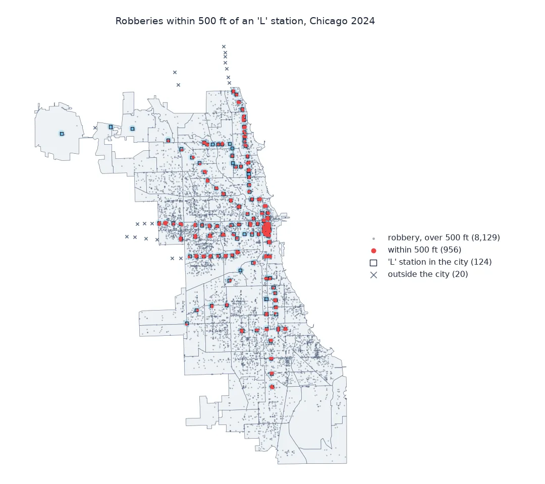
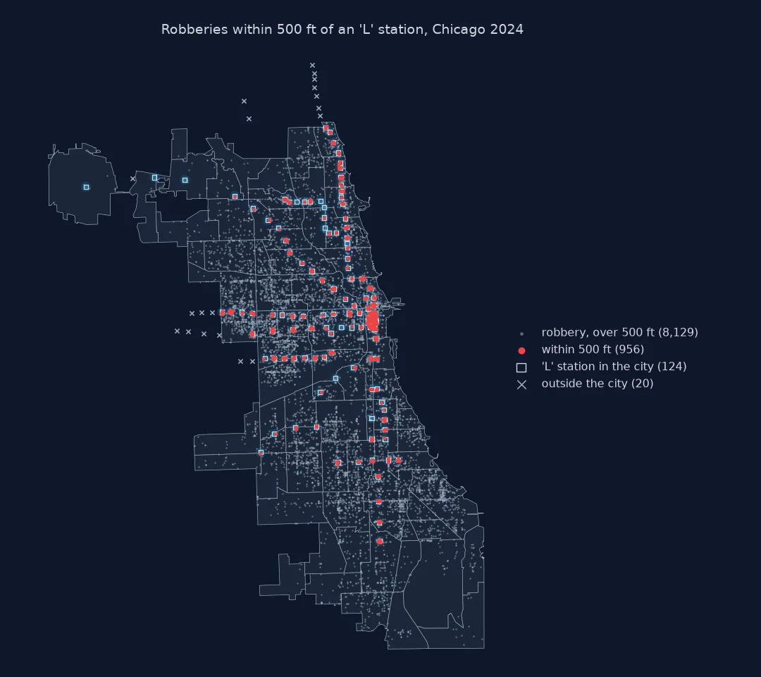
Stations inside coverage, density in rings, transit property
1. Keep stations inside the data's coverage
Chicago's crime data covers the city only, and the 'L' runs into Evanston, Skokie, Oak Park and other suburbs. A station whose surroundings are mostly outside the city will look safe because nothing outside is recorded:
print(f"{len(STATIONS)} stations; {STATIONS.inside.sum()} inside the city boundary")
print("outside:", ", ".join(sorted(STATIONS.loc[~STATIONS.inside, "name"].str.replace(r" \(.*", "", regex=True))))
144 stations; 124 inside the city boundary
outside: 54th/Cermak, Austin, Central, Cicero, Davis, Dempster, Dempster-Skokie , Forest Park, Foster, Harlem, Harlem/Lake, Linden, Main, Noyes, Oak Park, Oak Park, Oakton-Skokie, Ridgeland, Rosemont, South Boulevard
Twenty stations fall outside, among them the Purple Line in Evanston, the Yellow Line in Skokie, the western ends of the Blue and Green Lines in Oak Park and Forest Park, and stations such as Austin on the Blue Line that sit on the city line itself.
2. Measure density in rings
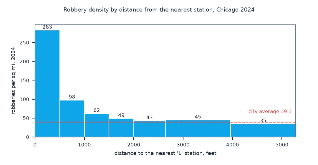
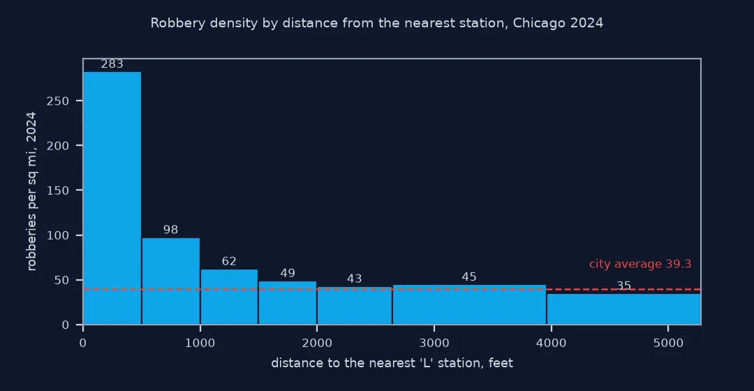
The ratio to the city average mixes two things: the station effect, and the fact that stations sit in dense, busy parts of the city. Density in rings around the stations shows how quickly it falls with distance:
rings = [0, 500, 1000, 1500, 2000, 2640, 3960, 5280]
rows = []
for lo, hi in zip(rings[:-1], rings[1:]):
    outer = ST.buffer(hi).union_all()
    band = (outer.difference(ST.buffer(lo).union_all()) if lo else outer).intersection(CITY)
    n = ((ROB.dist_ft >= lo) & (ROB.dist_ft < hi)).sum()
    rows.append({"ring (ft)": f"{lo:,}-{hi:,}", "robberies": n, "sq mi": round(band.area / SQ_MI, 2), "per sq mi": round(n / (band.area / SQ_MI), 1)})
R = pd.DataFrame(rows)
print(R.to_string(index=False))
print(f"city average: {len(ROB) / (CITY.area / SQ_MI):.1f} per sq mi")
ring (ft) robberies sq mi per sq mi
0-500 956 3.38 282.8
500-1,000 894 9.16 97.6
1,000-1,500 815 13.06 62.4
1,500-2,000 683 13.90 49.1
2,000-2,640 746 17.41 42.9
2,640-3,960 1338 29.78 44.9
3,960-5,280 793 22.64 35.0
city average: 39.3 per sq mi
Density falls by two thirds between the first ring and the second, from 282.8 to 97.6 robberies per square mile, and then flattens: from about 2,000 feet out it is close to the city average. The effect is concentrated within a block or two of the station.
3. Separate incidents on CTA property
Robberies on trains and platforms are recorded with a location description starting with "CTA". Their coordinates are often a station's, so they inflate the count next to stations:
ROB["on_cta"] = ROB.location_description.fillna("").str.startswith("CTA")
near = ROB.dist_ft <= 500
print(f"recorded on CTA property: {ROB.on_cta.mean():.1%} of all robberies, {ROB.on_cta[near].mean():.1%} of those within 500 ft")
off = ~ROB.on_cta
inner = R.loc[0, "sq mi"]
print(f"within 500 ft, not on CTA property: {(near & off).sum()} robberies, {(near & off).sum() / inner:.1f} per sq mi; "
      f"ring 2,640-3,960 ft: {R.loc[5, 'per sq mi']}")
recorded on CTA property: 6.0% of all robberies, 37.2% of those within 500 ft
within 500 ft, not on CTA property: 600 robberies, 177.5 per sq mi; ring 2,640-3,960 ft: 44.9
37.2% of the robberies within 500 feet are recorded on CTA property, against 6.0% city-wide: trains, platforms and stations. Without them the inner density is 177.5 per square mile, still four times the ring half a mile out, but well below 282.8.
Which stations, compared against what
The data used on this page
The City of Chicago's Crimes - 2001 to Present (ijzp-q8t2), robberies dated 2024 with coordinates; the CTA's List of 'L' Stops (8pix-ypme), with platforms grouped into stations by map_id; and the community area boundaries dissolved into the city outline. Distances are in US survey feet on EPSG:3435; 1,320 feet is a quarter mile.
from pathlib import Path

import geopandas as gpd
import numpy as np
import pandas as pd
import requests
from scipy.spatial import cKDTree

Path("data").mkdir(exist_ok=True)
URL = "https://data.cityofchicago.org/resource/ijzp-q8t2.json"
F = Path("data/chicago_crimes_2024.parquet")
if not F.exists():
    rows, offset = [], 0
    while True:
        part = requests.get(URL, timeout=300, params={
            "$where": "year=2024", "$limit": 50_000, "$offset": offset, "$order": "id",
            "$select": "id,date,primary_type,arrest,domestic,community_area,latitude,longitude,location_description,block,updated_on"}).json()
        rows += part; offset += len(part)
        if len(part) < 50_000:
            break
    pd.DataFrame(rows).to_parquet(F)
SRC = {"chicago_community_areas.geojson": "https://data.cityofchicago.org/resource/igwz-8jzy.geojson?$limit=100",
       "cta_l_stops.json": "https://data.cityofchicago.org/resource/8pix-ypme.json?$limit=1000"}
for name, url in SRC.items():
    if not Path("data", name).exists():
        Path("data", name).write_bytes(requests.get(url, timeout=120).content)

SQ_MI = 5280.0 ** 2
CITY = gpd.read_file("data/chicago_community_areas.geojson").to_crs(3435).union_all()
stops = pd.read_json("data/cta_l_stops.json")
stops["lat"] = stops.location.map(lambda p: float(p["latitude"]))
stops["lon"] = stops.location.map(lambda p: float(p["longitude"]))
s = stops.groupby("map_id").agg(name=("station_descriptive_name", "first"), lat=("lat", "mean"), lon=("lon", "mean")).reset_index()
STATIONS = gpd.GeoDataFrame(s, geometry=gpd.points_from_xy(s.lon, s.lat), crs=4326).to_crs(3435)
STATIONS["inside"] = STATIONS.within(CITY)
ST = STATIONS[STATIONS.inside].reset_index(drop=True)
r = pd.read_parquet(F).query("primary_type == 'ROBBERY'").dropna(subset=["latitude", "longitude"])
ROB = gpd.GeoDataFrame(r, geometry=gpd.points_from_xy(r.longitude.astype(float), r.latitude.astype(float)), crs=4326).to_crs(3435)
print(f"{len(stops)} platform stops in {len(STATIONS)} stations; {len(ROB):,} robberies with coordinates")
302 platform stops in 144 stations; 9,085 robberies with coordinates
Example 1: which stations, and against what
Rank stations by robberies within 500 feet, and set each against the density in its own ring at 2,640-3,960 feet, so a station is compared with its neighbourhood rather than with the city:
tree = cKDTree(np.c_[ROB.geometry.x, ROB.geometry.y])
xy = np.c_[ST.geometry.x, ST.geometry.y]
inner_n = np.array([len(p) for p in tree.query_ball_point(xy, 500)])
ring_n = np.array([len(p) for p in tree.query_ball_point(xy, 3960)]) - np.array([len(p) for p in tree.query_ball_point(xy, 2640)])
inner_a, ring_a = np.pi * 500 ** 2 / SQ_MI, np.pi * (3960 ** 2 - 2640 ** 2) / SQ_MI
T = pd.DataFrame({"station": ST.name.str.replace(r" \(.*", "", regex=True), "within_500ft": inner_n,
                  "local_ratio": (inner_n / inner_a) / (ring_n / ring_a)})
print(T.sort_values("within_500ft", ascending=False).head(6).round(1).to_string(index=False))
print(f"stations with no robbery within 500 ft: {(T.within_500ft == 0).sum()} of {len(T)}; median local ratio {T.local_ratio.median():.1f}")
station within_500ft local_ratio
Lake 35 8.1
Roosevelt 34 12.1
Harold Washington Library-State/Van Buren 33 7.3
Jackson 32 9.3
79th 30 16.3
69th 29 16.0
stations with no robbery within 500 ft: 11 of 124; median local ratio 3.3
Four of the top six are downtown Loop stations a few hundred feet apart, so their circles overlap and share incidents; the counts here are per station, not exclusive. Compared with their own surroundings, the South Side Red Line stations at 79th and 69th stand out most, at about 16 times their neighbourhood density. Eleven of the 124 stations had no robbery within 500 feet.
Routine activity theory at a station
Stations concentrate people at predictable times and places, which is the condition routine activity theory names for street crime: a motivated offender, a suitable target and no capable guardian, meeting. Robbery near stations follows that, but a buffer count on its own overstates it in two ways. Stations are built where the city is dense and busy, so part of any excess is the neighbourhood, not the station; comparing with rings further out, or with each station's own surroundings, separates the two. And incidents on trains and platforms are recorded at stations, so the inner ring collects offences that happened along the line.
The mechanics matter as much as the comparison. Buffers around nearby stations overlap downtown, so summing per-station counts counts some incidents twice; assigning each incident to its nearest station, or dissolving the buffers before measuring area, avoids that. Stations at the edge of the data's coverage look artificially quiet. And a quarter mile, the usual walking catchment, is too coarse to show an effect that is concentrated within a few hundred feet.
Centroids, bus stops and ridership
- Station centroids: platforms of one station are averaged; long stations, such as those spanning two blocks, have their incidents spread along the platform.
- Bus stops: CTA bus incidents ("CTA BUS", "CTA BUS STOP") are a separate pattern along bus routes.
- Ridership: robberies per million boardings is the transit agency's rate; CTA publishes daily station entries on the same portal.
- Network distance: walking distance along streets differs from straight-line distance where expressways and rail lines block the way.
- Border stations: stations on the city line, such as Austin on the Blue Line, have centroids just outside the boundary and are excluded with the suburban ones.
Internal links
- How to map crime hotspots with kernel density in Python — density without buffers
- How to calculate crime rates per resident in Python — rates and denominators
- How to map transit routes from GTFS in Python — transit data
FAQ
How do I count crimes near transit stations in Python?
Project both layers to a metric CRS, assign each incident to its nearest station with scipy.spatial.cKDTree.query, and count incidents within a radius; dissolve buffers before measuring area so overlaps are not counted twice.
Is crime higher near train stations?
In Chicago in 2024, robbery density within 500 feet of an 'L' station was 7.2 times the city average and 6.3 times the density half a mile to three quarters of a mile away; a third of those robberies were recorded on CTA property.
What radius should I use around stations?
Measure several: in Chicago the density fell by two thirds between the 0-500 ft and 500-1,000 ft rings, so a quarter-mile buffer dilutes the effect.
Why exclude stations outside the city?
The crime data covers only the city, so the area around a suburban station has no recorded incidents and would look safe.