
How to write a variable-rate prescription map
Problem statement
A prescription map is a polygon layer with a rate column, and the machine that reads it has opinions about all three words. The polygons must be simple, non-overlapping, and no finer than the implement can follow; the rate must be in the units the controller expects; and the file must be in a format and a coordinate system the terminal accepts.
Getting the agronomy right and the file wrong is the common outcome. The map loads, the controller applies a default rate everywhere, and nobody notices until the invoice for the fertiliser arrives.
This guide builds a prescription from zones, and gets the mechanical details right.
Quick answer
import geopandas as gpd, numpy as np

RATES = {0: 120.0, 1: 160.0, 2: 200.0}          # kg N/ha by zone

rx = zones.copy()
rx["rate"] = rx["zone"].map(RATES)
rx["rate_units"] = "kg/ha"
rx["product"] = "urea 46N"

rx = rx.to_crs(4326)                             # most terminals want WGS84
rx["geometry"] = rx.geometry.simplify(0.0001).buffer(0)
rx = rx[rx.geometry.is_valid & ~rx.geometry.is_empty]
rx = rx.explode(index_parts=False)
rx = rx[rx.to_crs(28992).area > 1000]            # drop fragments under 0.1 ha

assert rx["rate"].notna().all(), "some polygons have no rate"
assert not gpd.sjoin(rx, rx, predicate="overlaps").shape[0], "overlapping polygons"
rx.to_file("prescription.shp")                   # shapefile is the safest interchange
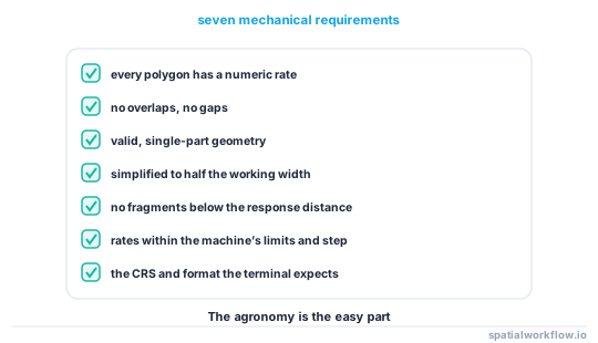
Three assertions before writing. Every one of them corresponds to a real failure in the field: a missing rate becomes zero or a default, an overlap makes the controller choose unpredictably, and a fragment smaller than the machine can respond to makes it oscillate.
Step-by-step solution
1. Decide the rates from something other than the zones
Zones say where the field differs; they do not say what rate to apply. The rate comes from an agronomic model, a nutrient balance, a soil test, or — best — an on-farm trial that measured the response. How to analyse an on-farm strip trial in Python covers the last.
2. Check the rates against the machine's limits
Every applicator has a minimum and a maximum rate and a rate resolution. A prescription outside those is clipped silently. Ask, and clip deliberately.
3. Simplify to the implement's resolution
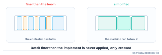
A spreader with a 24 m boom cannot follow a 5 m boundary, and a spinner's distribution pattern is several metres wide in any case. Simplifying at roughly half the working width removes detail that cannot be applied.
4. Remove fragments and slivers
A polygon smaller than the machine's response distance — speed times the actuator's lag, typically 5–15 m of travel — causes the rate to change and change back before it takes effect. Drop them into their neighbours.
5. Make the coverage clean
No overlaps, no gaps, valid geometry, single-part polygons. A gap gets the controller's default rate, which is usually not what you intended.
6. Write in the format the terminal reads
Shapefile is still the most widely accepted interchange. ISOXML (ISO 11783-10) is the standard for task data and is what most modern terminals prefer. Several manufacturers have their own formats. Ask before exporting, and test with a small file.
7. Report the totals before the file leaves
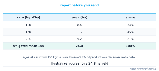
Area by rate, total product, and the average rate. A prescription that applies 40% more nitrogen than the uniform plan is a decision, and it should be a visible one.
Code examples
Example 1 — build the prescription with the checks
import numpy as np, geopandas as gpd

def build_prescription(zones, rates, product, units="kg/ha",
                       working_width_m=24, min_area_ha=0.1,
                       rate_limits=(0, 400), rate_step=None, crs_out=4326,
                       area_crs=28992):
    rx = zones.copy()
    rx["rate"] = rx["zone"].map(rates)

    missing = rx["rate"].isna().sum()
    if missing:
        raise ValueError(f"{missing} polygons have no rate")

    lo, hi = rate_limits
    clipped = ((rx["rate"] < lo) | (rx["rate"] > hi)).sum()
    rx["rate"] = rx["rate"].clip(lo, hi)
    if clipped:
        print(f"clipped {clipped} polygons to the machine limits {lo}–{hi}")
    if rate_step:
        rx["rate"] = (rx["rate"] / rate_step).round() * rate_step

    rx = rx.to_crs(area_crs)
    rx["geometry"] = rx.geometry.simplify(working_width_m / 2).buffer(0)
    rx = rx.explode(index_parts=False)
    before = len(rx)
    rx = rx[rx.area >= min_area_ha * 1e4]
    if before - len(rx):
        print(f"dropped {before - len(rx)} fragments under {min_area_ha} ha")

    rx["product"] = product
    rx["rate_units"] = units
    rx["area_ha"] = rx.area / 1e4

    overlaps = gpd.sjoin(rx, rx, predicate="overlaps")
    if len(overlaps):
        raise ValueError(f"{len(overlaps) // 2} overlapping polygon pairs")

    total = float((rx["rate"] * rx["area_ha"]).sum())
    print(rx.groupby("rate")["area_ha"].sum().round(2).to_string())
    print(f"total {total:,.0f} {units.split('/')[0]}; "
          f"area-weighted mean rate {total / rx['area_ha'].sum():.1f} {units}")
    return rx.to_crs(crs_out)
Example 2 — compare against the uniform plan
import numpy as np, pandas as pd

def compare_with_uniform(rx, uniform_rate, units="kg/ha"):
    area = rx["area_ha"].sum()
    variable = float((rx["rate"] * rx["area_ha"]).sum())
    flat = uniform_rate * area
    rows = rx.groupby("rate")["area_ha"].sum().reset_index()
    rows["share"] = rows["area_ha"] / area
    rows["vs_uniform"] = rows["rate"] - uniform_rate
    print(rows.round(2).to_string(index=False))
    print(f"\n{area:.1f} ha; variable {variable:,.0f} vs uniform {flat:,.0f} "
          f"({variable / flat - 1:+.1%})")
    return {"area_ha": area, "variable_total": variable, "uniform_total": flat,
            "difference_pct": variable / flat - 1}
Publishing the comparison is what turns a prescription from a black box into a decision. A variable plan that costs 15% more than the flat one may well be right; it should not be a surprise.
Example 3 — fill the gaps so the controller never uses a default
import geopandas as gpd

def fill_to_field(rx, field, default_rate, area_crs=28992):
    """Any part of the field with no polygon gets an explicit rate."""
    rx_m = rx.to_crs(area_crs)
    f = gpd.GeoDataFrame(geometry=[field], crs=rx.crs).to_crs(area_crs)
    gaps = gpd.overlay(f, rx_m[["geometry"]], how="difference").explode(index_parts=False)
    gaps = gaps[gaps.area > 100]
    if len(gaps):
        print(f"{len(gaps)} gaps totalling {gaps.area.sum()/1e4:.2f} ha "
              f"→ filling at {default_rate}")
        gaps["rate"] = default_rate
        gaps["product"] = rx_m["product"].iloc[0]
        gaps["rate_units"] = rx_m["rate_units"].iloc[0]
        rx_m = gpd.pd.concat([rx_m, gaps], ignore_index=True)
    return gpd.GeoDataFrame(rx_m, crs=area_crs).to_crs(rx.crs)
An explicit fill is always better than relying on the controller's default, because the default is a machine setting that somebody may have changed.
Explanation
Why detail finer than the implement is worse than useless
A boom sprayer with a 24 m width applies an average over that width; a spinner's pattern is wider still. A prescription boundary at 5 m resolution cannot be applied — and every boundary crossing costs the controller a rate change, which has a response lag. The result is a machine oscillating between rates while applying an average that has nothing to do with the map.
Why gaps are more dangerous than overlaps
An overlap is usually resolved by the controller taking the first or the last polygon, which is wrong in a small area. A gap falls through to the terminal's default rate, which may be zero, may be the last rate used, or may be a value somebody set for a different field. It is the one failure that can apply a completely unintended rate across a large area.
Why the shapefile persists
It is universally readable, it is simple enough that a terminal's embedded software can parse it, and every manufacturer has supported it for decades. Its limitations — ten-character field names, no real date type — barely matter for a file with three columns. ISOXML is the proper standard and is what modern terminals prefer, but shapefile remains the safest thing to hand somebody whose terminal you have not seen.
Why rate resolution matters
Applicators change rate in steps, and the step can be coarse — 10 kg/ha is common on older spreaders. A prescription with rates of 137 and 142 kg/ha is applied as the same rate, so the zones it distinguishes are not distinguished on the ground. Rounding to the machine's step before writing makes the map honest about what will happen.
Edge cases or notes
- Ask for the terminal's format first. Exporting blind wastes a field operation.
- Units differ by product. kg/ha, l/ha, seeds/m², thousand seeds/ha.
- Product form matters. 120 kg N/ha is not 120 kg/ha of urea.
- Shapefile truncates field names to ten characters.
- Most terminals want WGS84. Some want the local grid; ask.
- Headlands are often a separate rate, or excluded entirely.
- Test with one small file before a whole farm.
- Keep the as-applied data. It is the only evidence of what happened.
Internal links
- A prescription map is rejected by the machine controller — when the file will not load
- Management zones explained — where the polygons come from
- How to build management zones with clustering in Python — producing them
- How to analyse an on-farm strip trial in Python — where the rates should come from
- How to simplify geometry in GeoPandas — simplifying to the implement
- How to fix gaps and overlaps in a polygon coverage — making the coverage clean
- Shapefile column names are truncated — the ten-character limit
- How to package GIS deliverables in Python — what to hand over
FAQ
What format should a prescription map be in?
Ask the terminal. Shapefile is the most widely accepted interchange; ISOXML is the proper standard and what most modern terminals prefer.
How much should I simplify the polygons?
To about half the implement's working width. Finer detail cannot be applied and only makes the controller cross more boundaries.
What happens if my polygons have gaps?
The controller applies its default rate there, which may be zero or a value left from another field. Fill gaps explicitly.
Why does the machine apply the same rate to two different zones?
Because the applicator's rate resolution is coarser than the difference. Round the rates to the machine's step before writing.
Should I include the headland?
Usually as its own rate or excluded entirely — it is compacted, differently fertilised and turned on.
What should I check before exporting?
Every polygon has a rate, no overlaps, no fragments below the machine's response distance, valid single-part geometry, and the totals compared with the uniform plan.