
How to Make a GOES Satellite Loop in Python
On this page
Problem statement
The GOES-16 and GOES-18 satellites image the Americas every five minutes for the continental US sector, every ten for the full disk, and once a minute for the targeted mesoscale sectors. Every image is free on AWS. A loop of infrared images shows a hurricane's cloud tops boiling, the eye clearing and filling, and the storm's structure collapsing over land, which no single frame can. Getting there means finding the right files among thousands, reading a geostationary projection, cropping without reprojecting every frame, keeping one colour scale, and choosing a format that suits smooth imagery.
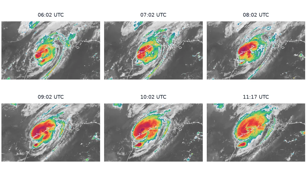
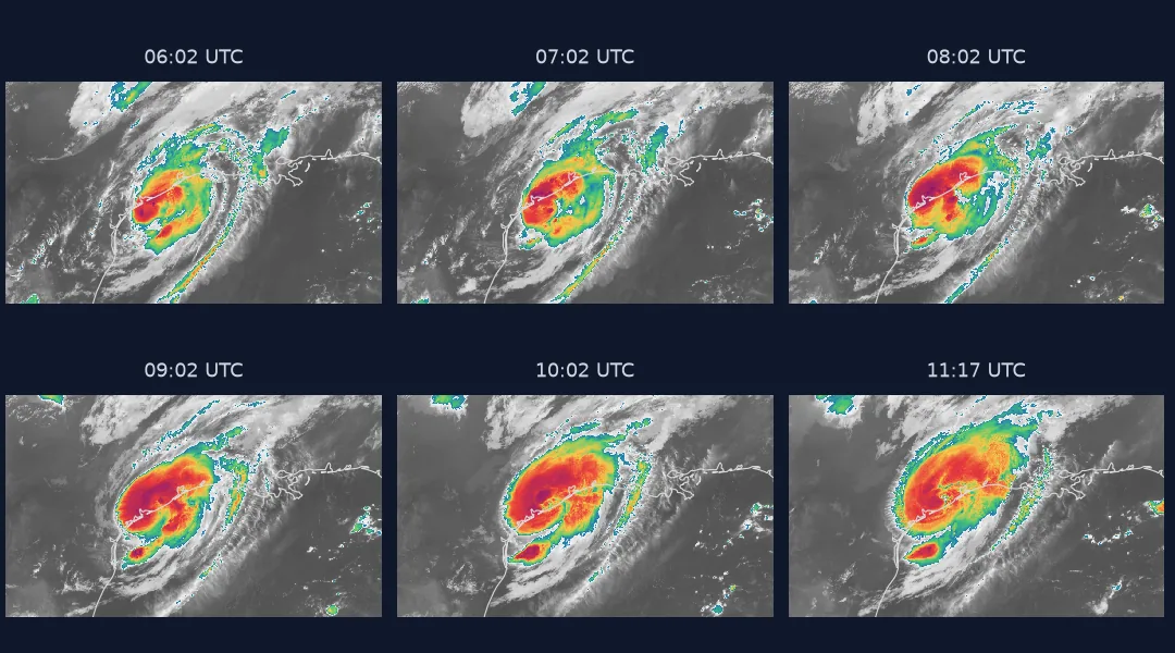
This page builds a six-hour infrared loop of Hurricane Beryl's landfall in Texas on 8 July 2024, from GOES-16 Advanced Baseline Imager band 13 (10.3 µm).
Quick answer
List the hour folders, take one file per 15 minutes, crop each frame in the satellite's native grid, and render with a fixed brightness-temperature colour scale:
frames = []
for key in KEYS:
    ds = xr.open_dataset(fetch(key), engine="h5netcdf")
    frames.append((pd.Timestamp(str(ds.t.values)), ds.CMI.values[np.ix_(IY, IX)]))          # brightness temperature, K
images = [render(a, t) for t, a in frames]
gap = pd.Series([t for t, _ in frames]).diff().dt.total_seconds().fillna(900).clip(upper=1800)
durations = (gap.shift(-1).fillna(900) / 900 * 250).round().astype(int).tolist()          # 15 min of storm = 250 ms
images[0].save("data/goes_beryl.webp", save_all=True, append_images=images[1:], duration=durations, loop=0, quality=80)
print(f"{len(frames)} frames {frames[0][0]:%H:%M}–{frames[-1][0]:%H:%M} UTC, each {frames[0][1].shape}, "
      f"{Path('data/goes_beryl.webp').stat().st_size / 1e6:.1f} MB")
24 frames 06:02–11:47 UTC, each (465, 787), 0.8 MB
Find files, read the geostationary grid, crop natively
1. Find the files
GOES products live in s3://noaa-goes16/<product>/<year>/<day of year>/<hour>/. Band 13 of the continental-US Cloud and Moisture Imagery is ABI-L2-CMIPC, file names containing M6C13, and 8 July 2024 is day 190:
print(f"{len(ALL_KEYS)} band-13 CONUS files between 06:00 and 12:00 UTC; kept {len(KEYS)} at 15-minute spacing")
starts = pd.Series([pd.to_datetime(re.search(r"_s(\d{13})", k).group(1), format="%Y%j%H%M%S") for k in KEYS])
gaps = starts.diff().dropna().dt.total_seconds() / 60
print("gaps between kept frames (min):", gaps.value_counts().sort_index().to_dict())
70 band-13 CONUS files between 06:00 and 12:00 UTC; kept 24 at 15-minute spacing
gaps between kept frames (min): {5.0: 1, 15.0: 21, 25.0: 1}
The archive is not perfect: one 15-minute slot has no scan, so two kept frames are 25 minutes apart. The loop gives that frame a longer duration, so the gap shows as a pause rather than a jump.
2. Read the geostationary grid
The image coordinates x and y are scan angles in radians from the satellite. Multiplied by the satellite height they become metres in a geostationary projection, which PROJ can convert:
p = ds0.goes_imager_projection
print(f"sub-satellite longitude {p.longitude_of_projection_origin}°, height {p.perspective_point_height:,.0f} m, sweep '{p.sweep_angle_axis}'")
print(f"full CONUS frame {ds0.CMI.shape}; crop {IY.sum()} x {IX.sum()} pixels "
      f"({IY.sum() * IX.sum() / ds0.CMI.size:.0%} of the frame)")
sub-satellite longitude -75.0°, height 35,786,023 m, sweep 'x'
full CONUS frame (1500, 2500); crop 465 x 787 pixels (10% of the frame)
3. Crop in the native grid, don't reproject every frame
Reprojecting each frame to latitude and longitude is slow and resamples the data. For a loop, crop the native grid to the box you want and draw coastlines transformed into the satellite's projection instead:
print(f"crop box in projection metres: x {EXT[0]:,.0f} to {EXT[1]:,.0f}, y {EXT[2]:,.0f} to {EXT[3]:,.0f}")
coast = land.to_crs(PROJ.crs)
print(f"coastline vertices transformed once: {sum(len(g.exterior.coords) for geom in coast.geometry for g in getattr(geom, 'geoms', [geom]))}")
crop box in projection metres: x -2,550,112 to -974,954, y 2,491,996 to 3,421,860
coastline vertices transformed once: 9842
4. Measure the storm through the loop
A fixed infrared scale also lets the frames be compared numerically. Cold cloud tops, below 200 K (−73 °C), mark the deepest convection around the eyewall:
bx, by = PROJ([-98, -93], [27, 31])
kx = (XC >= bx[0]) & (XC <= bx[1]); ky = (YC >= by[0]) & (YC <= by[1])
for t, a in frames[::4]:
    sub = a[np.ix_(ky, kx)]
    print(f"{t:%H:%M} UTC: coldest {np.nanmin(sub):.1f} K ({np.nanmin(sub) - 273.15:.0f} °C); below 200 K: {np.mean(sub < 200):.1%} of the box")
06:02 UTC: coldest 192.2 K (-81 °C); below 200 K: 0.7% of the box
07:02 UTC: coldest 191.9 K (-81 °C); below 200 K: 1.5% of the box
08:02 UTC: coldest 192.1 K (-81 °C); below 200 K: 5.1% of the box
09:02 UTC: coldest 194.8 K (-78 °C); below 200 K: 4.9% of the box
10:02 UTC: coldest 194.8 K (-78 °C); below 200 K: 3.4% of the box
11:12 UTC: coldest 197.9 K (-75 °C); below 200 K: 0.3% of the box
The area of very cold cloud peaks in the hour before landfall at about 08:40 UTC and shrinks afterwards, as the storm loses its ocean energy supply. The loop shows that collapse; the numbers confirm it.
5. Choose the format
images[0].save("data/goes_beryl.gif", save_all=True, append_images=images[1:], duration=durations, loop=0)
with imageio.get_writer("data/goes_beryl.mp4", format="FFMPEG", fps=4, codec="libx264", quality=7, macro_block_size=1) as w:
    for im in images:
        w.append_data(np.asarray(im))
for f in ("goes_beryl.gif", "goes_beryl.webp", "goes_beryl.mp4"):
    print(f"{f:16s} {Path('data', f).stat().st_size / 1e6:5.2f} MB")
goes_beryl.gif 2.75 MB
goes_beryl.webp 0.76 MB
goes_beryl.mp4 1.21 MB
Ranking formats for a GOES loop
The data used on this page
NOAA GOES-16 ABI Level 2 Cloud and Moisture Imagery, CONUS sector, band 13, 06:00–12:00 UTC on 8 July 2024, from the NOAA GOES archive on AWS; coastlines from Natural Earth 1:50m land.
import re
from pathlib import Path

import geopandas as gpd
import imageio.v2 as imageio
import matplotlib
matplotlib.use("Agg")
import matplotlib.pyplot as plt
import numpy as np
import pandas as pd
import requests
import xarray as xr
from matplotlib.colors import LinearSegmentedColormap
from PIL import Image
from pyproj import Proj

Path("data/goes").mkdir(parents=True, exist_ok=True)
B = "https://noaa-goes16.s3.amazonaws.com/"
ALL_KEYS = []
for h in range(6, 12):
    text = requests.get(B, params={"list-type": 2, "prefix": f"ABI-L2-CMIPC/2024/190/{h:02d}/OR_ABI-L2-CMIPC-M6C13"}, timeout=60).text
    ALL_KEYS += re.findall(r"<Key>([^<]+)</Key>", text)
slot = lambda k: pd.to_datetime(re.search(r"_s(\d{11})", k).group(1), format="%Y%j%H%M").floor("15min")
KEYS = list(pd.Series(ALL_KEYS).groupby([slot(k) for k in ALL_KEYS]).first())      # first scan in each 15-min slot


def fetch(key):
    path = Path("data/goes", key.split("/")[-1])
    if not path.exists():
        path.write_bytes(requests.get(B + key, timeout=300).content)
    return path


if not Path("data/ne_50m_land.zip").exists():
    Path("data/ne_50m_land.zip").write_bytes(requests.get("https://naciscdn.org/naturalearth/50m/physical/ne_50m_land.zip", timeout=300).content)
ds0 = xr.open_dataset(fetch(KEYS[0]), engine="h5netcdf")
p = ds0.goes_imager_projection
PROJ = Proj(proj="geos", h=p.perspective_point_height, lon_0=p.longitude_of_projection_origin, sweep=p.sweep_angle_axis,
            a=p.semi_major_axis, b=p.semi_minor_axis)
x, y = ds0.x.values * p.perspective_point_height, ds0.y.values * p.perspective_point_height
bx, by = PROJ([-102, -86, -102, -86], [24, 24, 34, 34])
IX, IY = (x >= min(bx)) & (x <= max(bx)), (y >= min(by)) & (y <= max(by))
XC, YC = x[IX], y[IY]
EXT = (XC.min(), XC.max(), YC.min(), YC.max())
land = gpd.read_file("data/ne_50m_land.zip").cx[-110:-80, 20:40]
CMAP = LinearSegmentedColormap.from_list("ir", [(0.0, "#2b0a3d"), (0.10, "#8e1b6e"), (0.18, "#e83b3b"), (0.26, "#f7c948"),
                                                (0.34, "#48c774"), (0.42, "#1f78b4"), (0.43, "#f2f2f2"), (1.0, "#101010")])


def render(a, when):
    fig = plt.figure(figsize=(5, 3), dpi=100)
    ax = fig.add_axes([0, 0, 1, 1]); ax.set_axis_off()
    ax.imshow(a, cmap=CMAP, vmin=180, vmax=320, extent=EXT, interpolation="nearest")
    land.to_crs(PROJ.crs).boundary.plot(ax=ax, color="#d9d9d9", linewidth=0.4)
    ax.set_xlim(EXT[0], EXT[1]); ax.set_ylim(EXT[2], EXT[3])
    ax.text(0.02, 0.95, f"GOES-16 band 13  {when:%H:%M} UTC", transform=ax.transAxes, color="white", fontsize=8, va="top")
    fig.canvas.draw(); im = Image.fromarray(np.asarray(fig.canvas.buffer_rgba())).convert("RGB")
    plt.close(fig)
    return im


print(f"{len(ALL_KEYS)} files listed, {len(KEYS)} kept")
70 files listed, 24 kept
Example 1: compare with the radar loop's format ranking
sizes = {f: Path("data", f).stat().st_size for f in ("goes_beryl.gif", "goes_beryl.webp", "goes_beryl.mp4")}
order = sorted(sizes, key=sizes.get)
print("smallest to largest:", order)
print(f"distinct colours in one frame: {len(np.unique(np.asarray(images[8]).reshape(-1, 3), axis=0)):,}")
smallest to largest: ['goes_beryl.webp', 'goes_beryl.mp4', 'goes_beryl.gif']
distinct colours in one frame: 771
A fixed grid of scan angles, not a map projection
Geostationary satellites sit 35,786 km above the equator and scan the same view again and again. That is what makes loops possible. Their images come on a fixed grid of scan angles, not on a map projection most software expects. For a loop the native grid is an advantage: every frame has the same pixels, so cropping is just array slicing and the frames line up exactly. Only the overlays need to be transformed, once, into the satellite's projection.
Infrared brightness temperature is a continuous field with smooth gradients, so even after rendering a frame has hundreds of distinct colours, 771 in the one measured here, more than GIF's 256. That reverses the format ranking seen with radar loops. GIF must quantise each frame to 256 colours, which bands the gradients and costs bytes. Video codecs and WebP compress smooth imagery efficiently. Measure on your own frames; the right answer depends on the picture.
Mid-scan times, sector changes and parallax
- Mid-scan time: the
tvariable is the middle of the scan; file names carry start and end times. - Missing scans happen; pace by timestamps or mark the gap.
- Sector changes: mesoscale sectors move with the weather; the CONUS sector does not.
- GOES-East moved: GOES-19 replaced GOES-16 as GOES-East in 2025; later dates use the
noaa-goes19bucket. - Visible bands are dark at night; band 13 infrared works around the clock.
- Parallax: high cloud tops appear displaced away from the sub-satellite point; it matters when overlaying radar or ground data.
Internal links
- How to make a weather radar loop — the ground-based counterpart
- How to map a hurricane track from IBTrACS — the track behind the loop
FAQ
How do I download GOES-16 imagery in Python?
List https://noaa-goes16.s3.amazonaws.com/?list-type=2&prefix=ABI-L2-CMIPC/<year>/<doy>/<hour>/ with requests, filter on the band (M6C13), and download the NetCDF files; no account is needed.
How do I georeference GOES ABI images?
Multiply the x and y scan angles by the satellite height and use a PROJ geos projection with the file's longitude_of_projection_origin and sweep axis.
Should I reproject satellite frames for an animation?
Usually not: crop in the native grid and transform overlays instead. Every frame keeps identical pixels and no resampling is needed.
What format is best for a satellite loop?
For smooth infrared imagery, WebP or MP4 are usually much smaller than GIF; measure on your frames.