Time-Series Maps Explained: Events, Tracks, Snapshots and Fields

On this page

Problem statement

"A map that changes over time" covers very different data. An earthquake catalogue is a list of events, each with one place and one moment. A hurricane best track is one object moving, sampled every few hours. A weekly drought map is a sequence of snapshots of areas. A satellite or radar archive is a continuous field sampled on a grid at irregular instants. Each kind has its own natural time step, its own way of filling the gaps between samples, and its own mistakes when it is turned into frames. Treating them all as "frames of a map" is how events get counted twice and storms jump.

This page sorts temporal geodata into four kinds and measures the time step of real datasets of each kind. It then shows what each kind needs before it can be mapped over time.

Quick answer

Identify the kind of data first, because it decides how time is handled:

Kind	Example	Time is…	Between samples	Typical mistake
Events	earthquakes	a property of each point	nothing happens	showing an event in more than one frame
Tracks	hurricane best track	a sequence along one object	interpolate the path	joining points in file order instead of time order
Snapshots	weekly drought areas	a label on each layer	the state holds until the next one	classifying each snapshot separately
Fields	radar, satellite, sea ice	the scan or averaging time	unknown; do not invent	treating irregular scans as regular

Then measure the data's own time step before choosing a frame step:

for name, times in STEPS.items():
    gaps = np.diff(np.sort(times.to_numpy())).astype("timedelta64[s]").astype(float)
    print(f"{name:28s} {len(times):>5,} times, step median {pretty(np.median(gaps)):>9}, range {pretty(gaps.min())}–{pretty(gaps.max())}")

earthquakes (Ridgecrest)     2,451 times, step median   1.2 min, range 0 s–20.1 h
hurricane track (Beryl)        109 times, step median     3.0 h, range 20.0 min–3.0 h
drought snapshots (Texas)       54 times, step median     7.0 d, range 7.0 d–7.0 d
radar scans (KHGX)              95 times, step median   1.8 min, range 1.2 min–3.4 min
sea ice (September means)       47 times, step median    1.0 yr, range 1.0 yr–1.0 yr

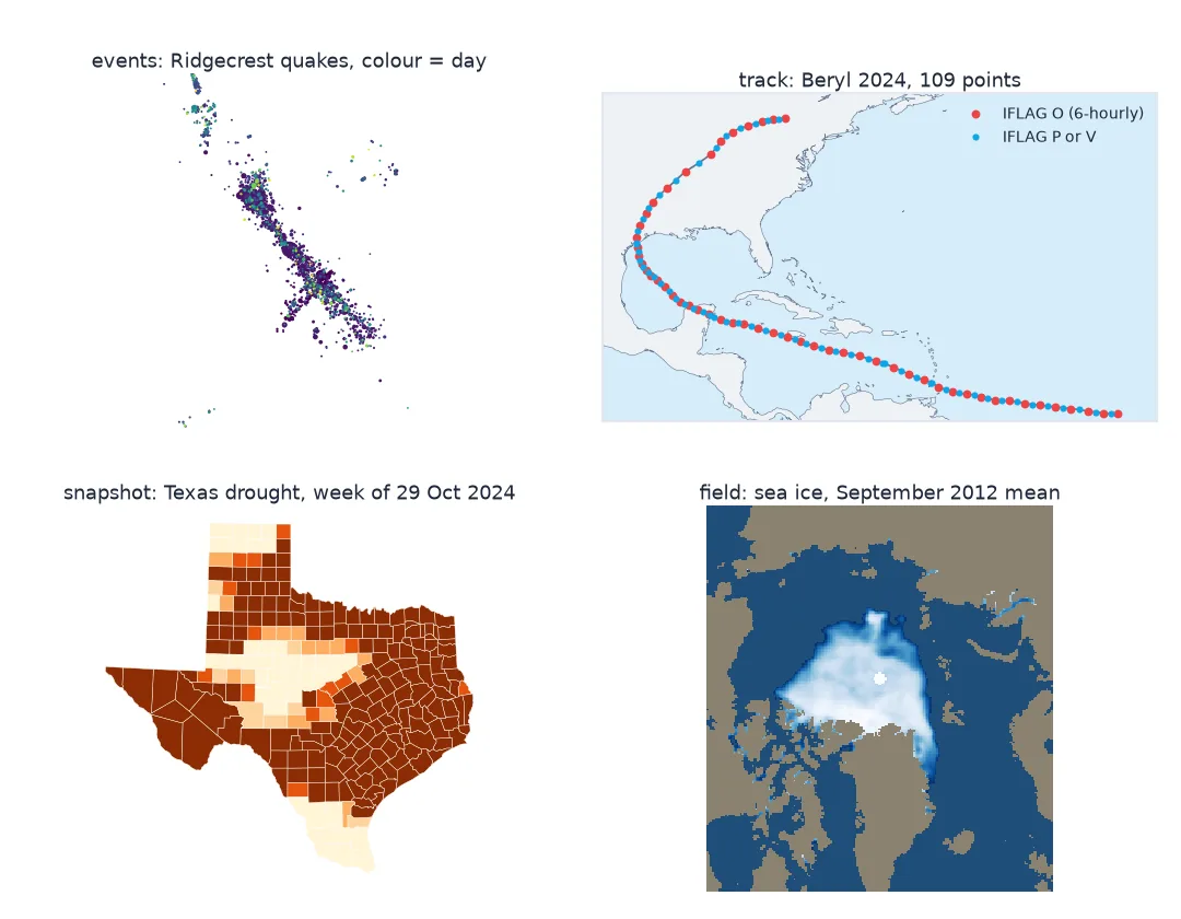
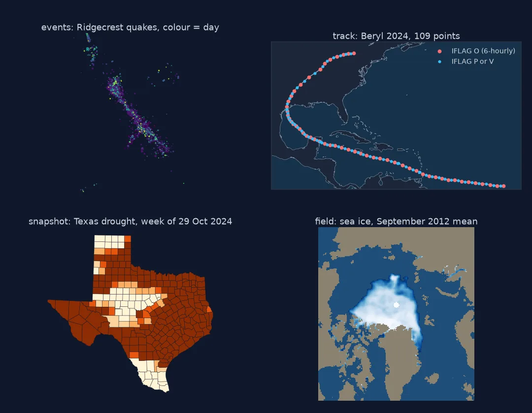
Four maps: Ridgecrest earthquakes as points coloured by day; Hurricane Beryl's 2024 track with original six-hourly points in red and other points in blue; Texas counties coloured by drought class for the week of 29 October 2024; and Arctic sea ice concentration for September 2012. — Four kinds of time-series geodata from this cluster: events, a track, a snapshot and a field. Each handles time differently.

Events, tracks, snapshots and fields, each with its clock

1. Events: decide how long each one stays on the map

An event has a moment, not a duration. Any time window that frames them is your choice: a frame of "the past 24 hours" or "everything so far". The window decides what the map claims, so state it, and make sure an event is counted once per window:

q = STEPS["earthquakes (Ridgecrest)"]
for window in ("1h", "1D"):
    per = q.dt.floor(window).value_counts()
    print(f"{window:>3} windows: {len(per)} non-empty, busiest {per.max()} events, median {per.median():.0f}")

 1h windows: 404 non-empty, busiest 199 events, median 2
 1D windows: 28 non-empty, busiest 1239 events, median 29

2. Tracks: order by time and know the sampling

A track is only a line if its points are in time order. Its sampling is not constant either, and not all of its points are original fixes. Look at both:

gaps_min = np.diff(np.sort(STEPS["hurricane track (Beryl)"].to_numpy())).astype("timedelta64[m]").astype(int)
print("Beryl track gaps (minutes):", pd.Series(gaps_min).value_counts().sort_index().to_dict())
t = pd.to_datetime(beryl.ISO_TIME)
print(f"on six-hourly synoptic times: {((t.dt.hour % 6 == 0) & (t.dt.minute == 0)).sum()}; "
      f"IFLAG first letter: {beryl.IFLAG.str[0].value_counts().to_dict()}; special records: {beryl.USA_RECORD.str.strip().replace('', np.nan).dropna().tolist()}")

Beryl track gaps (minutes): {20: 2, 45: 1, 60: 1, 120: 1, 135: 1, 160: 2, 180: 100}
on six-hourly synoptic times: 53; IFLAG first letter: {'O': 53, 'P': 52, 'V': 4}; special records: ['L', 'I', 'L', 'L']

A best track mixes original fixes with filled-in points; know which is which before drawing them as equals.

3. Snapshots: the state holds until the next one

A weekly drought map describes conditions over a week. Between two maps there is no new information. Show each snapshot for its whole validity period, and keep one classification for all of them, as the flicker fix shows.

4. Fields: sampled, not continuous

A radar or satellite field exists everywhere, but it is sampled only at scan times, and the scan spacing can change mid-sequence. A frame per scan plays at a changing speed unless frame durations follow the gaps. Averaged fields such as monthly sea-ice grids are a different case: each value is a mean over the month, so there is no single instant to place it at.

Frame steps that suit five datasets

The data used on this page

Times from five datasets used in this cluster: the USGS ComCat catalogue for Ridgecrest, July 2019 (M2.5+); IBTrACS v04r01 for Hurricane Beryl, 2024; the US Drought Monitor weekly statistics for Texas, 2024; KHGX radar scan times on 8 July 2024 from the Unidata Level III archive; and the NSIDC Sea Ice Index September extent table.

import re
from pathlib import Path

import numpy as np
import pandas as pd
import requests

Path("data").mkdir(exist_ok=True)
SRC = {
    "ridgecrest_2019.csv": ("https://earthquake.usgs.gov/fdsnws/event/1/query?format=csv&starttime=2019-07-01&endtime=2019-08-01"
                            "&minlatitude=35.3&maxlatitude=36.2&minlongitude=-118.0&maxlongitude=-117.2&minmagnitude=2.5&orderby=time-asc"),
    "ibtracs.NA.list.v04r01.csv": "https://www.ncei.noaa.gov/data/international-best-track-archive-for-climate-stewardship-ibtracs/v04r01/access/csv/ibtracs.NA.list.v04r01.csv",
    "N_09_extent_v4.0.csv": "https://noaadata.apps.nsidc.org/NOAA/G02135/north/monthly/data/N_09_extent_v4.0.csv",
}
for name, url in SRC.items():
    if not Path("data", name).exists():
        Path("data", name).write_bytes(requests.get(url, timeout=600).content)
if not Path("data/tx_county_2024.csv").exists():
    Path("data/tx_county_2024.csv").write_text(requests.get(
        "https://usdmdataservices.unl.edu/api/CountyStatistics/GetDroughtSeverityStatisticsByAreaPercent",
        params={"aoi": "TX", "startdate": "1/1/2024", "enddate": "12/31/2024", "statisticsType": 1},
        headers={"Accept": "text/csv"}, timeout=120).text)

quakes = pd.read_csv("data/ridgecrest_2019.csv")
ib = pd.read_csv("data/ibtracs.NA.list.v04r01.csv", skiprows=[1], low_memory=False, keep_default_na=False)
beryl = ib[(ib.NAME == "BERYL") & (ib.SEASON.astype(int) == 2024)]
usdm = pd.read_csv("data/tx_county_2024.csv")
L3 = "https://unidata-nexrad-level3.s3.amazonaws.com/"
keys = []
for hour in ("08", "09", "10"):
    keys += re.findall(r"<Key>([^<]+)</Key>", requests.get(L3, params={"list-type": 2, "prefix": f"HGX_N0B_2024_07_08_{hour}_"}, timeout=60).text)
ice = pd.read_csv("data/N_09_extent_v4.0.csv", skipinitialspace=True)
ice = ice[ice["year"] <= 2025]                     # 1979–2025: NSIDC appends each new September

STEPS = {
    "earthquakes (Ridgecrest)": pd.to_datetime(quakes.time, utc=True),
    "hurricane track (Beryl)": pd.to_datetime(beryl.ISO_TIME),
    "drought snapshots (Texas)": pd.Series(pd.to_datetime(usdm.MapDate.astype(str)).unique()),
    "radar scans (KHGX)": pd.Series(pd.to_datetime([k[-19:] for k in keys], format="%Y_%m_%d_%H_%M_%S")),
    "sea ice (September means)": pd.Series(pd.to_datetime(ice["year"].astype(str) + "-09-15")),
}


def pretty(seconds):
    for unit, size in (("yr", 365 * 86400), ("d", 86400), ("h", 3600), ("min", 60)):
        if seconds >= size:
            return f"{seconds / size:.1f} {unit}"
    return f"{seconds:.0f} s"


print({k: len(v) for k, v in STEPS.items()})

{'earthquakes (Ridgecrest)': 2451, 'hurricane track (Beryl)': 109, 'drought snapshots (Texas)': 54, 'radar scans (KHGX)': 95, 'sea ice (September means)': 47}

Example 1: frame steps that suit each dataset

suggest = {"earthquakes (Ridgecrest)": "1 h windows, fading", "hurricane track (Beryl)": "1 h, interpolated",
           "drought snapshots (Texas)": "1 week, one per map", "radar scans (KHGX)": "one per scan, paced by gaps",
           "sea ice (September means)": "1 year, one per mean"}
for name, times in STEPS.items():
    span = (times.max() - times.min()).total_seconds()
    print(f"{name:28s} spans {pretty(span):>9}; frame step: {suggest[name]}")

earthquakes (Ridgecrest)     spans    27.3 d; frame step: 1 h windows, fading
hurricane track (Beryl)      spans    13.0 d; frame step: 1 h, interpolated
drought snapshots (Texas)    spans    1.0 yr; frame step: 1 week, one per map
radar scans (KHGX)           spans     3.0 h; frame step: one per scan, paced by gaps
sea ice (September means)    spans   46.0 yr; frame step: 1 year, one per mean

The roles time plays in geodata

Time enters geodata in different roles. For events, time is an attribute: the map at time t is a filter on the events, and the frame window is a choice. For tracks, time orders the vertices of a moving object: the map at time t is an interpolated position. For snapshots, time labels a whole layer valid for a period: the map at time t is whichever layer is valid then. For fields, time is the sampling instant (or the averaging period) of a grid: the map at time t is the nearest sample, and the reader should know how near.

What a frame means depends on the kind of data, and so does the step it should use.

The measured steps show why one recipe cannot fit all. Earthquakes arrive seconds to hours apart, irregularly. Beryl's track is three-hourly, but only the 53 six-hourly points carry IBTrACS's "original" flag. The 52 points in between are flagged otherwise, and four extra points mark three landfalls and the intensity peak. Drought maps are exactly weekly, radar scans change spacing within an hour, and the sea-ice series is one average per year. Each guide in this cluster starts by measuring this step, then chooses frames that show it honestly.

Mixed kinds, validity periods and gaps

One typical mistake per kind of temporal data.

Mixed kinds: a hurricane map often combines a track (the storm), fields (rain) and snapshots (warnings); give each its own time logic.
Validity periods: snapshot data usually carries valid-from and valid-to dates (the Drought Monitor's ValidStart, ValidEnd); use them rather than the map date alone.
Averages have no instant; label them with their period ("September 2012"), not a date.
Time zones affect all four kinds; keep UTC until the label.
Gaps: missing samples should leave visible gaps, not be filled silently.

Internal links

Animated maps explained — what motion can and cannot show
How to animate an earthquake sequence — events
How to animate a hurricane track — tracks
How to make an animated drought map — snapshots
How to make a radar loop animation — fields

FAQ

What is a time-series map?

A map of data that changes over time, shown as an animation, a set of small multiples, a slider or a change map.

What kinds of temporal data can a map show?

Events (points in time), tracks (moving objects), snapshots (areas valid for a period) and fields (gridded samples). Each needs its own handling of time.

How do I choose the time step for an animated map?

Measure the data's own step first: event spacing, track sampling, snapshot period or scan interval. Then choose a frame step that does not invent detail the data lacks.

Can I interpolate between time steps?

For tracks, yes: the path between fixes is a reasonable assumption. For snapshots and fields, interpolating invents data; show the nearest sample instead.