
How to Measure Land Cover Along Streams in Python
On this page
Problem statement
The strip of land along a stream, the riparian zone, does more for water quality than its size suggests: trees there shade the water, hold the banks and filter runoff before it reaches the channel. Planning rules and studies measure it with buffers of a fixed width, often 30 m or 100 m, and ask how much of the buffer is forest or developed. Done by buffering each stream segment and summing, the answer double-counts every confluence and every pair of parallel channels, because neighbouring buffers overlap.
This page measures land cover by distance from streams in Williamson County, Texas, using the USGS National Hydrography Dataset (NHD) and NLCD 2021. It uses a distance transform, so every pixel is counted once, in exactly one distance band.
Quick answer
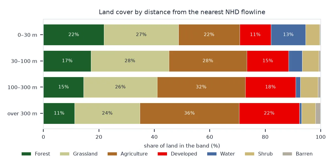
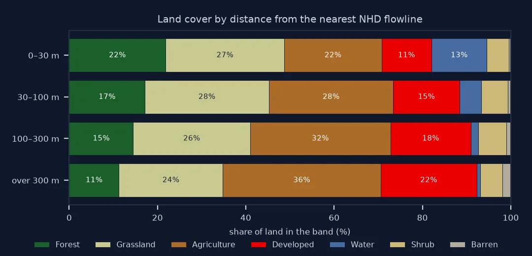
Rasterise the streams onto the land cover grid, compute each pixel's distance to the nearest stream, and cross-tabulate distance bands against classes:
streams = features.rasterize([(g, 1) for g in FLOW.geometry], out_shape=LC.shape, transform=TRANSFORM, all_touched=True)
dist = ndimage.distance_transform_edt(streams == 0) * 30           # metres, pixel centre to nearest stream pixel
bands = pd.cut(dist[LC > 0], [-1, 30, 100, 300, np.inf], labels=["0–30 m", "30–100 m", "100–300 m", "over 300 m"])
groups = pd.Series(LC[LC > 0]).map(GROUP)
table = pd.crosstab(pd.Series(bands, name="distance"), groups.rename("group"), normalize="index") * 100
print(table[["Forest", "Developed", "Grassland", "Agriculture", "Water"]].round(1).to_string())
group Forest Developed Grassland Agriculture Water
distance
0–30 m 21.8 11.3 26.9 22.0 12.6
30–100 m 17.1 15.0 28.1 28.2 4.9
100–300 m 14.5 18.2 26.5 31.8 1.7
over 300 m 11.3 21.8 23.5 35.8 0.8
Forest makes up 22% of the land within 30 m of a stream and 11% beyond 300 m; agriculture and developed land rise with distance from the water.
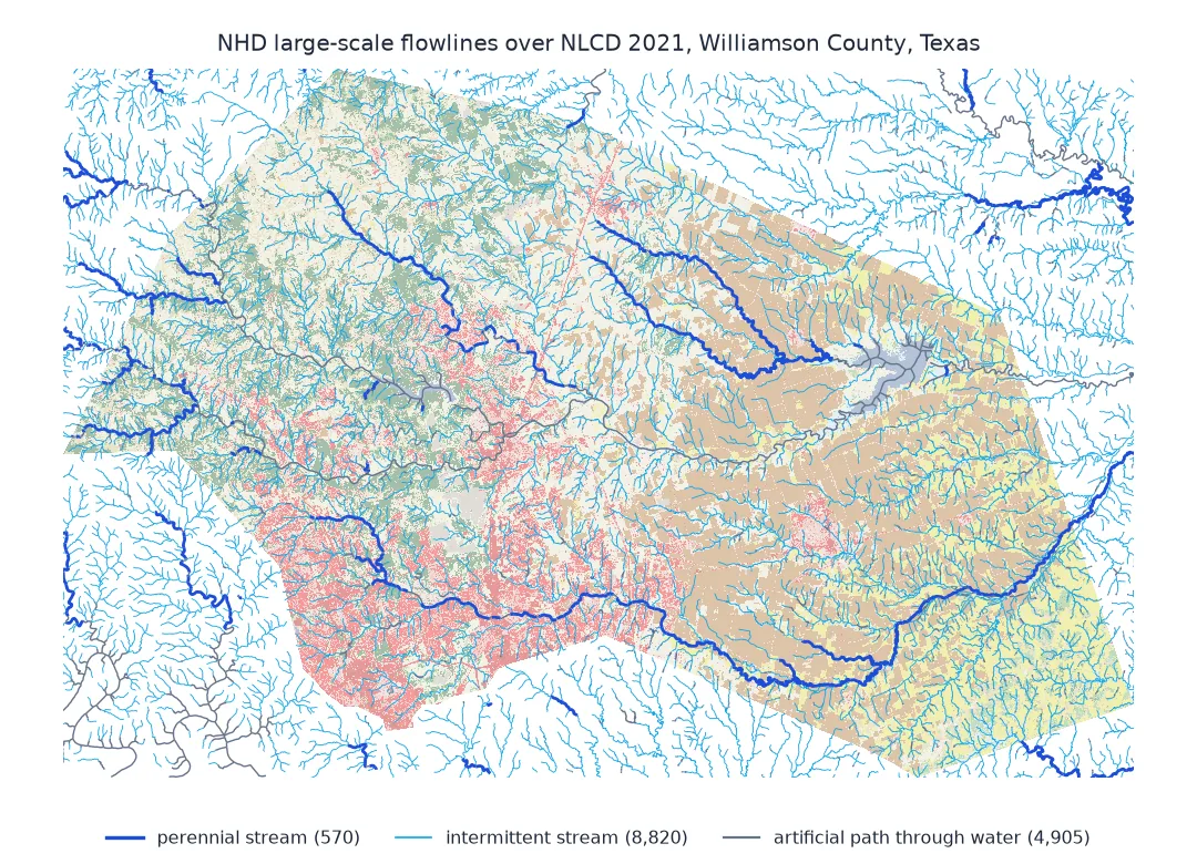
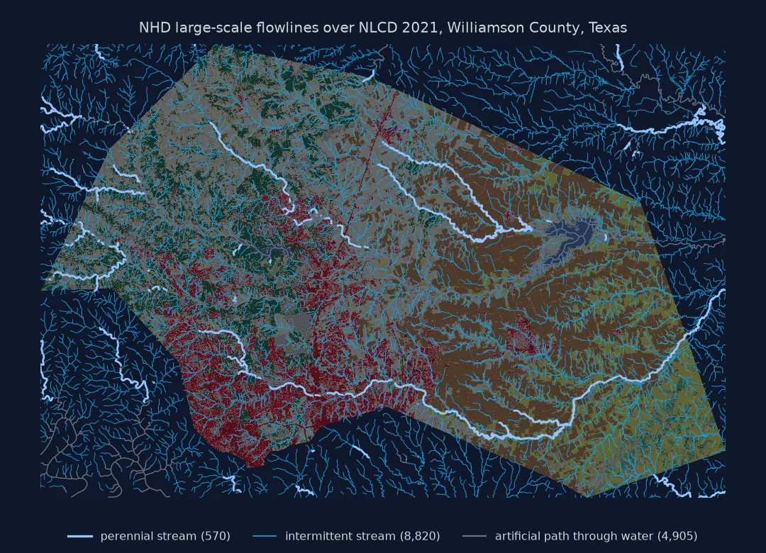
Which lines are streams, no summed buffers, perennial and intermittent
1. Know which lines are streams
NHD flowlines include artificial paths drawn through lakes, canals and pipelines, and streams with intermittent or ephemeral flow. The feature code says which:
FCODES = {46006: "stream, perennial", 46003: "stream, intermittent", 46007: "stream, ephemeral", 55800: "artificial path (through water bodies)",
          42807: "pipeline", 33400: "connector", 33600: "canal/ditch"}
print(FLOW.fcode.map(FCODES).fillna("other").value_counts().to_string())
print(f"total length: {FLOW.length.sum() / 1000:,.0f} km")
fcode
stream, intermittent 8820
artificial path (through water bodies) 4905
stream, perennial 570
pipeline 80
connector 10
canal/ditch 5
total length: 7,182 km
Artificial paths carry the network through lakes; with the lake already in the land cover as water, they add little. Pipelines are not streams at all.
2. Do not sum buffer areas
Buffering each segment and adding the areas counts overlaps once per segment:
streams_only = FLOW[FLOW.fcode.isin([46006, 46003, 46007])]
buf = streams_only.buffer(30)
print(f"30 m buffers: summed {buf.area.sum() / 1e6:,.1f} km², dissolved {buf.union_all().area / 1e6:,.1f} km² "
      f"({buf.area.sum() / buf.union_all().area - 1:+.0%})")
30 m buffers: summed 410.3 km², dissolved 388.3 km² (+6%)
3. Compare perennial and intermittent streams
Distances to different kinds of stream need separate rasters:
rows = {}
for name, codes in (("perennial", [46006]), ("intermittent", [46003])):
    s = features.rasterize([(g, 1) for g in FLOW[FLOW.fcode.isin(codes)].geometry], out_shape=LC.shape, transform=TRANSFORM, all_touched=True)
    near = (ndimage.distance_transform_edt(s == 0) * 30 <= 30) & (LC > 0)
    rows[name] = pd.Series(LC[near]).map(GROUP).value_counts(normalize=True) * 100
print(pd.DataFrame(rows).loc[["Forest", "Developed", "Agriculture", "Grassland"]].round(1).to_string())
perennial intermittent
Forest 28.7 21.6
Developed 7.0 12.0
Agriculture 7.7 24.1
Grassland 17.5 28.5
Perennial streams are lined with more forest and less farmland than intermittent ones, which run through fields and pasture for much of their length.
Riparian forest in numbers
The data used on this page
Flowlines from the USGS National Hydrography Dataset large-scale map service (layer 6), paged 2,000 at a time for the bounding box of Williamson County, Texas (saved on 11 October 2026 and read from a copy on this site, since the service's answer changed between runs), and NLCD 2021 (30 m) from MRLC's WCS masked to the 2023 Census county outline, all in CONUS Albers (EPSG:5070).
import io
import json
import time
import zipfile
from pathlib import Path

import geopandas as gpd
import numpy as np
import pandas as pd
import rasterio
import rasterio.mask
import requests
from rasterio import features
from scipy import ndimage

Path("data").mkdir(exist_ok=True)
if not Path("data/cb_2023_us_county_20m.zip").exists():
    Path("data/cb_2023_us_county_20m.zip").write_bytes(requests.get("https://www2.census.gov/geo/tiger/GENZ2023/shp/cb_2023_us_county_20m.zip", timeout=300).content)
COUNTY = gpd.read_file("data/cb_2023_us_county_20m.zip").query("GEOID == '48491'").to_crs(5070)
lon0, lat0, lon1, lat1 = COUNTY.to_crs(4326).total_bounds
F = Path("data/williamson_flowlines.geojson")
if not F.exists():
    # A copy of the NHD flowlines saved on 2026-10-11 (14,390). The live query it stands for:
    # feats, offset = [], 0
    # while True:
    #     page = requests.get("https://hydro.nationalmap.gov/arcgis/rest/services/nhd/MapServer/6/query",
    #                         params={"geometry": f"{lon0},{lat0},{lon1},{lat1}", "geometryType": "esriGeometryEnvelope", "inSR": 4326,
    #                                 "spatialRel": "esriSpatialRelIntersects", "outFields": "gnis_name,fcode,lengthkm", "outSR": 4326,
    #                                 "orderByFields": "OBJECTID", "resultOffset": offset, "resultRecordCount": 2000, "f": "geojson"}, timeout=300).json()
    #     feats += page["features"]
    #     offset += len(page["features"])
    #     if len(page["features"]) < 2000:
    #         break
    # F.write_text(json.dumps({"type": "FeatureCollection", "features": feats}))
    reply = requests.get("https://data.spatialworkflow.io/nhd-williamson-flowlines-2026-10-11.zip", timeout=300)
    reply.raise_for_status()
    with zipfile.ZipFile(io.BytesIO(reply.content)) as z:
        z.extract("williamson_flowlines.geojson", "data")
FLOW = gpd.read_file(F).to_crs(5070)
path = Path("data/nlcd_2021.tif")
if not path.exists():
    x0, y0, x1, y1 = COUNTY.total_bounds
    for attempt in range(4):
        r = requests.get("https://www.mrlc.gov/geoserver/mrlc_download/wcs", params={"service": "WCS", "version": "2.0.1", "request": "GetCoverage",
                         "coverageId": "mrlc_download__NLCD_2021_Land_Cover_L48", "subset": [f"X({x0},{x1})", f"Y({y0},{y1})"], "format": "image/geotiff"}, timeout=300)
        if r.status_code < 500:
            break
        time.sleep(15 * (attempt + 1))
    r.raise_for_status()
    path.write_bytes(r.content)
with rasterio.open(path) as src:
    lc, TRANSFORM = rasterio.mask.mask(src, COUNTY.geometry, crop=True, nodata=0)
LC = lc[0]
GROUP = {11: "Water", 90: "Water", 95: "Water", 21: "Developed", 22: "Developed", 23: "Developed", 24: "Developed", 31: "Barren",
         41: "Forest", 42: "Forest", 43: "Forest", 52: "Shrub", 71: "Grassland", 81: "Agriculture", 82: "Agriculture"}
print(f"{len(FLOW):,} NHD flowlines; NLCD {LC.shape[1]} x {LC.shape[0]} pixels")
14,390 NHD flowlines; NLCD 2845 x 1884 pixels
Example 1: riparian forest in numbers
near = (dist <= 30) & (LC > 0)
forest = np.isin(LC, [41, 42, 43])
print(f"land within 30 m of a flowline: {near.sum() * 900 / 1e6:,.0f} km² ({near.sum() / (LC > 0).sum():.1%} of the county), "
      f"holding {(near & forest).sum() / forest.sum():.0%} of the county's forest")
land within 30 m of a flowline: 368 km² (12.6% of the county), holding 18% of the county's forest
Buffers overlap at every junction
A buffer is a distance band around a feature. When features are many and close together, as stream networks are, buffers overlap at every junction, and a polygon overlay counts the overlap once per feature unless the buffers are dissolved first. A distance transform avoids the problem: it assigns every pixel its distance to the nearest stream pixel, so the bands partition the landscape exactly once, and composition by band is a single cross-tabulation.
The resolution sets the precision. On a 30 m grid a "30 m buffer" is one or two pixels either side of the stream line, and all_touched=True makes every pixel the line crosses a stream pixel, so the innermost band is approximate. For narrow buffers, use a finer grid or a vector overlay of dissolved buffers with the land cover polygons. For bands of 100 m and wider, the raster approach is both exact enough and far faster.
Edges, artificial paths and banks
- Edge effects: streams just outside the download box are missing; pad the flowline query by the widest band.
- Stream density: NHD large scale maps far more small intermittent channels than medium scale; results depend on which.
- Artificial paths run through lakes and reservoirs; keep or drop them deliberately.
- Banks, not centrelines: wide rivers have banks well away from their centreline; for them, measure from the water body polygon.
- Distance metric:
distance_transform_edtgives Euclidean distance in pixels; multiply by the pixel size.
Internal links
- How to measure land cover around points — buffers around points
- How to measure impervious surface by watershed — the same streams' watersheds
FAQ
How do I calculate land cover in a riparian buffer?
Rasterise the stream lines, compute each pixel's distance to the nearest stream with scipy.ndimage.distance_transform_edt, and cross-tabulate distance bands against land cover classes.
Why is my buffer area larger than the area it covers?
Overlapping buffers were summed. Dissolve them first, or use a distance raster, which counts each pixel once.
Where can I get stream lines for the US?
The USGS National Hydrography Dataset, as downloads or through its map service; flowline layer 6 is the large-scale network.
What do NHD feature codes 46006 and 46003 mean?
46006 is a perennial stream, 46003 an intermittent one; 55800 is an artificial path through a water body.