How to Download NLCD Land Cover for an Area in Python

On this page

Problem statement

The National Land Cover Database (NLCD) maps the contiguous United States in 30 m pixels and 16 classes, for nine years between 2001 and 2021. The national files are several gigabytes each, and most analyses need one county or one watershed. The Multi-Resolution Land Characteristics consortium (MRLC), which publishes NLCD, also serves it through a Web Coverage Service (WCS): ask for a box, get a GeoTIFF of exactly those pixels, with no account and no key.

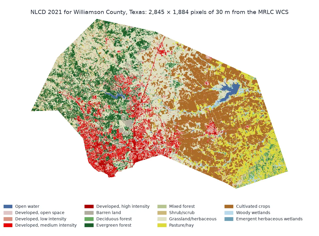
This page downloads NLCD 2001 and 2021 for Williamson County, Texas, one of the fastest-growing counties in the country. It checks that the pixels arrive on the national grid, unresampled, and turns them into class areas.

Quick answer

Project the area's boundary to the NLCD's CRS (CONUS Albers, EPSG:5070), request its bounding box with GetCoverage, and mask:

def nlcd(year, bounds, path):
    if not Path(path).exists():
        x0, y0, x1, y1 = bounds
        for attempt in range(4):                       # the server answers 502 now and then: retry with a pause
            r = requests.get(WCS, params={"service": "WCS", "version": "2.0.1", "request": "GetCoverage",
                                          "coverageId": f"mrlc_download__NLCD_{year}_Land_Cover_L48",
                                          "subset": [f"X({x0},{x1})", f"Y({y0},{y1})"], "format": "image/geotiff"}, timeout=300)
            if r.status_code < 500:
                break
            time.sleep(15 * (attempt + 1))
        r.raise_for_status()
        Path(path).write_bytes(r.content)
    return path

with rasterio.open(nlcd(2021, COUNTY.total_bounds, "data/nlcd_2021.tif")) as src:
    lc, transform = rasterio.mask.mask(src, COUNTY.geometry, crop=True, nodata=0)
lc = lc[0]
print(f"{lc.shape[1]} x {lc.shape[0]} pixels; {(lc > 0).sum() * 900 / 1e6:,.0f} km² inside the county")

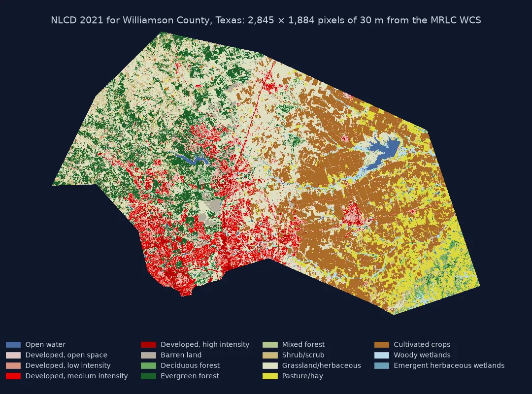
2845 x 1884 pixels; 2,926 km² inside the county

Land cover map of Williamson County, Texas, in 2021 in the official NLCD colours: developed land in reds concentrated in the south-west around Round Rock, Cedar Park and Georgetown, evergreen forest and grassland in the hilly west, cultivated crops and pasture across the flat east, and Granger Lake as a blue shape in the east. — Williamson County in NLCD 2021, cut from the national map by one WCS request.

Find coverages, check the grid, turn pixels into areas

1. Find the coverages

The service's capabilities document lists every coverage. The land cover layers for the lower 48 states follow one naming pattern:

caps = requests.get(WCS, params={"service": "WCS", "version": "2.0.1", "request": "GetCapabilities"}, timeout=120).text
ids = sorted(set(re.findall(r"<wcs:CoverageId>(mrlc_download__NLCD_(\d{4})_Land_Cover_L48)</wcs:CoverageId>", caps)))
print("NLCD land cover years:", [y for _, y in ids])

NLCD land cover years: ['2001', '2004', '2006', '2008', '2011', '2013', '2016', '2019', '2021']

2. Check the grid

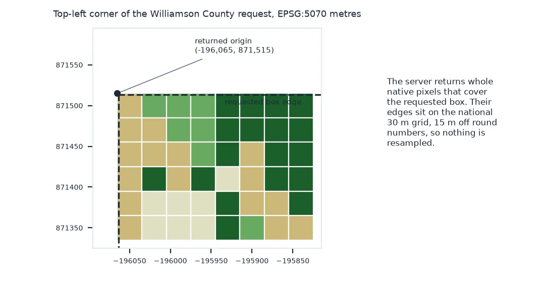
A WCS request is a box in map coordinates, and a server could resample to fit it. This one does not: it returns the native pixels that cover the box. Check that the origin of what came back sits on the national 30 m grid:

with rasterio.open("data/nlcd_2021.tif") as src:
    t = src.transform
    print(f"pixel size {t.a:.0f} x {-t.e:.0f} m; origin ({t.c:,.0f}, {t.f:,.0f})")
    print(f"offset from the national grid origin (-2,493,045, 3,310,005): {(t.c + 2493045) % 30:.0f} m, {(3310005 - t.f) % 30:.0f} m")
    print("palette entry for class 23:", src.colormap(1)[23])

pixel size 30 x 30 m; origin (-196,065, 871,515)
offset from the national grid origin (-2,493,045, 3,310,005): 0 m, 0 m
palette entry for class 23: (235, 0, 0, 255)

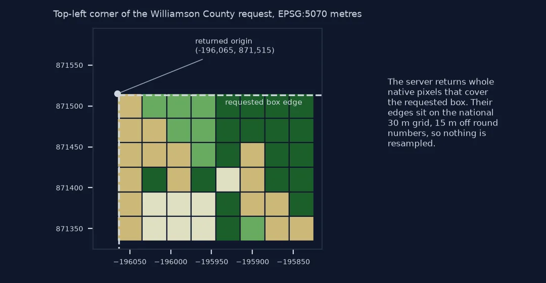
The grid edges fall 15 m off round numbers (…045, …005), so a box drawn on round coordinates still gets whole native pixels. Requesting an output CRS other than EPSG:5070 would make the server reproject, and categorical pixels should not be resampled by anyone but you.

Close-up of the top-left corner of the downloaded raster: coloured 30 metre pixels whose top-left corner sits at minus 196,065 and 871,515 in EPSG:5070 metres, slightly outside the dashed edge of the requested box. — The server returns whole native pixels covering the request; their edges stay on the national grid.

3. Turn pixels into areas

Each pixel is 30 m × 30 m = 900 m² in an equal-area projection, so class areas are counts times 900:

values, counts = np.unique(lc[lc > 0], return_counts=True)
areas = pd.Series(counts * 900 / 1e6, index=[NLCD_CLASSES[v] for v in values]).sort_values(ascending=False)
print(areas.round(1).head(6).to_string())

Grassland/herbaceous     757.8
Cultivated crops         639.7
Evergreen forest         314.3
Pasture/hay              272.2
Developed, open space    170.3
Shrub/scrub              167.0

The same county in 2001

The data used on this page

National Land Cover Database 2001 and 2021 (lower 48 states, 30 m) from MRLC's WCS service, and the Williamson County, Texas outline from the 2023 Census cartographic boundary files.

import re
import time
from pathlib import Path

import geopandas as gpd
import numpy as np
import pandas as pd
import rasterio
import rasterio.mask
import requests

Path("data").mkdir(exist_ok=True)
WCS = "https://www.mrlc.gov/geoserver/mrlc_download/wcs"
if not Path("data/cb_2023_us_county_20m.zip").exists():
    Path("data/cb_2023_us_county_20m.zip").write_bytes(requests.get("https://www2.census.gov/geo/tiger/GENZ2023/shp/cb_2023_us_county_20m.zip", timeout=300).content)
COUNTY = gpd.read_file("data/cb_2023_us_county_20m.zip").query("GEOID == '48491'").to_crs(5070)
NLCD_CLASSES = {11: "Open water", 12: "Perennial ice/snow", 21: "Developed, open space", 22: "Developed, low intensity",
                23: "Developed, medium intensity", 24: "Developed, high intensity", 31: "Barren land", 41: "Deciduous forest",
                42: "Evergreen forest", 43: "Mixed forest", 52: "Shrub/scrub", 71: "Grassland/herbaceous", 81: "Pasture/hay",
                82: "Cultivated crops", 90: "Woody wetlands", 95: "Emergent herbaceous wetlands"}
print(f"{COUNTY.NAME.iloc[0]} County, Texas: {COUNTY.area.iloc[0] / 1e6:,.0f} km², bounds {COUNTY.total_bounds.round(0)}")

Williamson County, Texas: 2,926 km², bounds [-196063.  814997. -110723.  871514.]

Example 1: the same county in 2001

with rasterio.open(nlcd(2001, COUNTY.total_bounds, "data/nlcd_2001.tif")) as src:
    lc01 = rasterio.mask.mask(src, COUNTY.geometry, crop=True, nodata=0)[0][0]
dev = [21, 22, 23, 24]
d01, d21 = np.isin(lc01, dev).sum() * 900 / 1e6, np.isin(lc, dev).sum() * 900 / 1e6
print(f"developed land: {d01:,.0f} km² in 2001, {d21:,.0f} km² in 2021 ({d21 / d01 - 1:+.0%})")

developed land: 332 km² in 2001, 523 km² in 2021 (+58%)

A Web Coverage Service cuts what you ask for

A Web Coverage Service is the raster counterpart of a feature service: you describe the part of a coverage you want, and the server cuts it from the full dataset. For NLCD it is the practical way to work on a region without handling national files. The service returns the stored pixels, in the stored CRS, with the colour palette embedded, so what you receive is the same data you would cut from the national GeoTIFF yourself.

Five steps from a county name to class areas.

The checks matter because land cover is categorical. A resampled pixel is a new value with no class behind it, or a class shifted to the wrong place. Requesting in the native CRS and verifying the grid origin ensures every pixel is an original classification. Area calculations are then simple, because CONUS Albers is equal-area and every pixel covers the same 900 m².

Years, Alaska and Hawaii, and size limits

NLCD download problems and fixes.

Years: NLCD 2001, 2004, 2006, 2008, 2011, 2013, 2016, 2019 and 2021 from the 2021 release are consistent with each other; do not mix years from different releases.
Alaska, Hawaii and Puerto Rico have separate coverages (_AK, _HI, _PR) and fewer years.
Size limits and errors: very large boxes may be refused or slow, and the server returns an occasional 502 under load; request tiles, retry with a pause, and check that each file opens.
Impervious surface is served the same way (NLCD_2021_Impervious_L48), as a percentage per pixel.
Annual NLCD (1985–2023) is a newer product; the WCS here serves its change summaries, not the yearly maps.

Internal links

Land cover products explained — NLCD among the other land cover maps
How to calculate zonal statistics in Python — summarising rasters by polygon

FAQ

How do I download NLCD data in Python?

Request a bounding box in EPSG:5070 from MRLC's WCS with GetCoverage and the coverage id mrlc_download__NLCD_<year>_Land_Cover_L48, then read the GeoTIFF with rasterio.

What resolution is NLCD?

30 m, in CONUS Albers Equal Area (EPSG:5070), so each pixel covers 900 m².

Which years does NLCD cover?

The 2021 release covers 2001, 2004, 2006, 2008, 2011, 2013, 2016, 2019 and 2021.

Does the NLCD WCS resample the data?

Not when you request the native CRS: it returns whole native pixels covering your box, aligned to the national grid.