How to Recreate John Snow's Cholera Map in Python

On this page

Problem statement

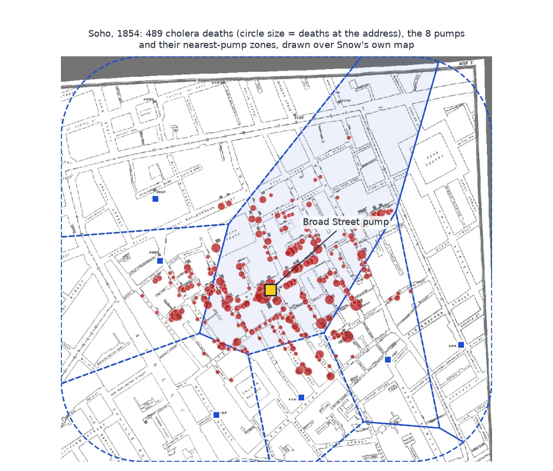
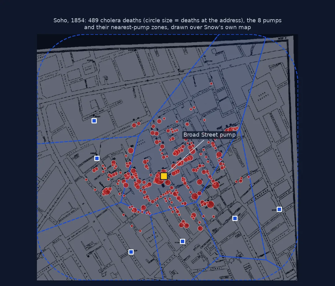
In September 1854 cholera killed hundreds of people in a few streets of Soho, London. John Snow mapped the deaths, house by house, and the map showed them clustered around one water pump on Broad Street. It is the best-known map in epidemiology, and the data behind it are small enough to analyse completely: 489 deaths at 250 addresses and the 8 public pumps of the area, digitised and georeferenced by Robin Wilson.

This page loads that data in GeoPandas, assigns every death to its nearest pump, measures how the deaths fall off with distance from Broad Street, and draws the result over Snow's own map.

Quick answer

Read the deaths and pumps, find each address's nearest pump, and add up the deaths per pump:

dist = np.column_stack([DEATHS.distance(p) for p in PUMPS.geometry])   # metres, British National Grid
DEATHS["nearest_pump"] = dist.argmin(axis=1)
per_pump = DEATHS.groupby("nearest_pump").Count.sum().reindex(range(len(PUMPS)), fill_value=0)
print(f"{DEATHS.Count.sum()} deaths at {len(DEATHS)} addresses; nearest pump (straight line):")
print(per_pump.rename(index=PUMP_NAMES).to_string())
print(f"share nearest Broad Street: {per_pump[0] / per_pump.sum():.1%}")

489 deaths at 250 addresses; nearest pump (straight line):
nearest_pump
Broad Street    340
pump 1           65
pump 2            5
pump 3            0
pump 4           40
pump 5           27
pump 6            0
pump 7           12
share nearest Broad Street: 69.5%

Snow's 1854 map of Soho as a faded background, with red circles at 250 addresses sized by the number of cholera deaths, the eight pumps as blue squares, the Broad Street pump highlighted in yellow, and dashed nearest-pump zones; the shaded Broad Street zone contains most of the deaths, which crowd around the pump. — The digitised deaths and pumps over Snow's own map. Most deaths fall in the zone nearest the Broad Street pump.

Expand the counts, draw pump catchments, measure the fall-off

1. Expand the counts

Each point is an address with a count of deaths, from 1 to 15. Statistics about people need the counts as weights, or a house with 15 deaths counts the same as one with 1:

print(DEATHS.Count.value_counts().sort_index().to_string())
print(f"addresses with more than one death: {(DEATHS.Count > 1).sum()} holding {DEATHS.Count[DEATHS.Count > 1].sum()} deaths")

Count
1     136
2      56
3      26
4      18
5       9
7       1
8       3
15      1
addresses with more than one death: 114 holding 353 deaths

2. Draw the pump catchments

Thiessen (Voronoi) polygons divide the area into the zones nearest each pump, the view Snow himself drew around Broad Street:

area = box(*DEATHS.total_bounds).buffer(150)
cells = shapely.voronoi_polygons(MultiPoint(list(PUMPS.geometry)), extend_to=area)
catch = gpd.GeoDataFrame({"pump": range(len(PUMPS))}, geometry=[next(c for c in cells.geoms if c.contains(p)).intersection(area) for p in PUMPS.geometry], crs=27700)
catch["deaths"] = catch.pump.map(per_pump)
catch["deaths_per_ha"] = catch.deaths / (catch.area / 1e4)
print(catch.assign(name=catch.pump.map(PUMP_NAMES))[["name", "deaths", "deaths_per_ha"]].round(2).to_string(index=False))

        name  deaths  deaths_per_ha
Broad Street     340          26.90
      pump 1      65           9.97
      pump 2       5           0.38
      pump 3       0           0.00
      pump 4      40           8.56
      pump 5      27           7.76
      pump 6       0           0.00
      pump 7      12           1.78

3. Measure the fall-off with distance

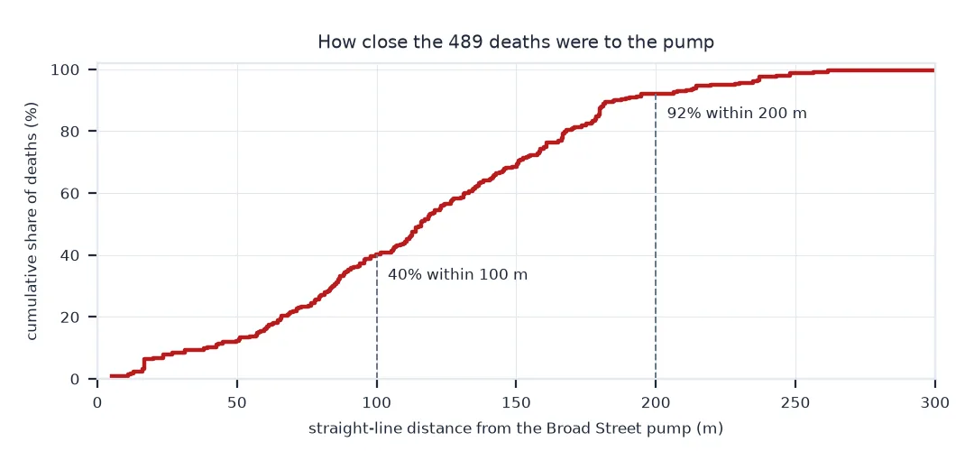
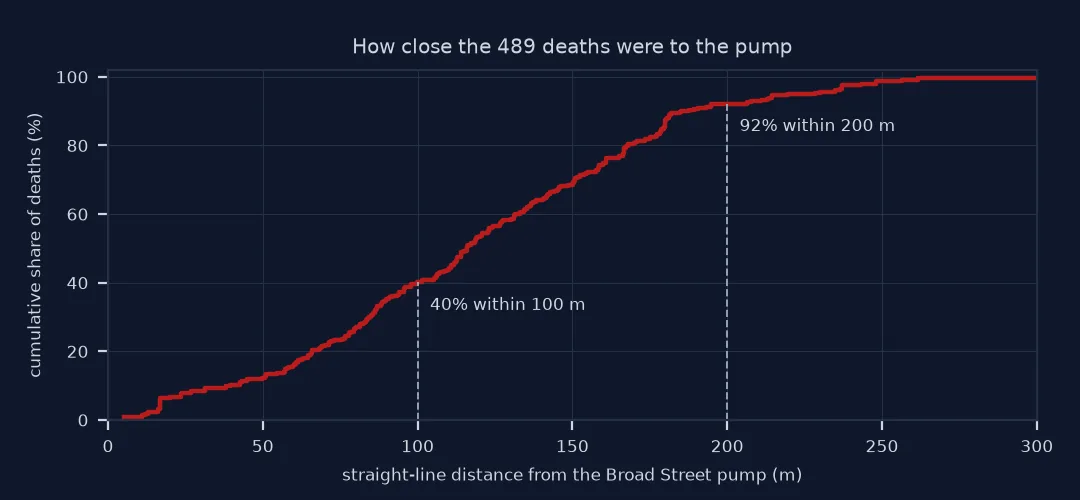
If the Broad Street pump was the source, deaths should concentrate near it and thin out with distance:

d_bs = dist[:, 0]
for r in (50, 100, 150, 200, 250):
    print(f"within {r:3d} m of Broad Street: {DEATHS.Count[d_bs <= r].sum():3d} deaths ({DEATHS.Count[d_bs <= r].sum() / DEATHS.Count.sum():.0%})")
cx = np.average(DEATHS.geometry.x, weights=DEATHS.Count); cy = np.average(DEATHS.geometry.y, weights=DEATHS.Count)
print(f"death-weighted mean centre: {np.hypot(cx - PUMPS.geometry.x[0], cy - PUMPS.geometry.y[0]):.0f} m from the Broad Street pump")

within  50 m of Broad Street:  60 deaths (12%)
within 100 m of Broad Street: 196 deaths (40%)
within 150 m of Broad Street: 335 deaths (69%)
within 200 m of Broad Street: 451 deaths (92%)
within 250 m of Broad Street: 483 deaths (99%)
death-weighted mean centre: 19 m from the Broad Street pump

Step chart of the cumulative share of the 489 deaths against straight-line distance from the Broad Street pump: 40 percent within 100 metres, 92 percent within 200 metres, and nearly all within 260 metres. — Deaths fall off steeply with distance from the pump.

Deaths by walking distance to the next pump

The data used on this page

Robin Wilson's SnowGIS layers: cholera deaths per address and the pumps, digitised from Snow's 1854 map and georeferenced to the British National Grid (EPSG:27700), with Snow's map itself as a georeferenced GeoTIFF. The Broad Street pump is identified as the pump 2.7 m from the memorial pump's position in Wikidata.

from pathlib import Path

import geopandas as gpd
import numpy as np
import pandas as pd
import requests
import shapely
from shapely.geometry import MultiPoint, Point, box

Path("data").mkdir(exist_ok=True)
Z = Path("data/SnowGIS_v2.zip")
if not Z.exists():
    Z.write_bytes(requests.get("https://www.rtwilson.com/downloads/SnowGIS_v2.zip", timeout=300).content)
DEATHS = gpd.read_file(f"zip://{Z}!SnowGIS/Cholera_Deaths.shp")
PUMPS = gpd.read_file(f"zip://{Z}!SnowGIS/Pumps.shp")
H = {"User-Agent": "spatialworkflow.io guide (info@spatialworkflow.io)"}
memorial = requests.get("https://www.wikidata.org/wiki/Special:EntityData/Q139765546.json", headers=H, timeout=60).json()
c = memorial["entities"]["Q139765546"]["claims"]["P625"][0]["mainsnak"]["datavalue"]["value"]
m = gpd.GeoSeries([Point(c["longitude"], c["latitude"])], crs=4326).to_crs(27700).iloc[0]
bs = int(PUMPS.distance(m).idxmin())
PUMPS = pd.concat([PUMPS.loc[[bs]], PUMPS.drop(index=bs)]).reset_index(drop=True)      # Broad Street first
PUMP_NAMES = {0: "Broad Street", **{k: f"pump {k}" for k in range(1, len(PUMPS))}}
print(f"CRS {DEATHS.crs.to_string()}; {len(DEATHS)} addresses, {DEATHS.Count.sum()} deaths, {len(PUMPS)} pumps; "
      f"Broad Street pump {PUMPS.distance(m).min():.1f} m from the memorial")

CRS EPSG:27700; 250 addresses, 489 deaths, 8 pumps; Broad Street pump 2.7 m from the memorial

Example 1: deaths by walking towards the next pump

Points nearer another pump still died in large numbers if Broad Street was only a little further; compare distances for the deaths assigned elsewhere:

other = DEATHS.nearest_pump != 0
extra = dist[other, 0] - dist[other].min(axis=1)
print(f"{DEATHS.Count[other].sum()} deaths nearer another pump; Broad Street was on average {np.average(extra, weights=DEATHS.Count[other]):.0f} m further for them")

149 deaths nearer another pump; Broad Street was on average 64 m further for them

Why Snow's map works as evidence

Snow's map works because of the design of the evidence: individual cases at their addresses, every pump marked, and a hypothesis that predicts a pattern. If cholera came from the Broad Street pump, deaths should cluster around it, and they do: most of the deaths are nearer that pump than any other, and the centre of the deaths is a few tens of metres from it. Snow also used exceptions, such as the brewery workers who drank beer and stayed well, and households far away who had fetched Broad Street water by preference.

Deaths assigned to their nearest pump.

Straight-line distance is a simplification Snow himself refined: people walked along streets, and his later map drew the area around Broad Street by walking distance. Thiessen polygons on a dense street grid such as Soho's are a fair first approximation; around a large block, walking distance can be very different. The digitised data also inherit the original map's choices: deaths are drawn as stacked bars at addresses, so positions are building fronts, and only deaths are recorded, not the people at risk.

Counts, no denominator and pump identity

Snow data traps.

Counts, not cases: each point is an address; use Count as a weight in every statistic.
No denominator: Snow's map shows deaths, not rates; population per house is unknown, so density reflects housing too.
CRS: the data are in British National Grid (EPSG:27700), metres; distances are straight-line.
Pump identity: the file carries no names; locating Broad Street against a known position avoids relying on file order.
Historical map: SnowMap.tif is Snow's map warped to the modern grid, good for display rather than measurement.

Internal links

How to make a kernel density map of disease cases — the same deaths as a surface
How to create Voronoi service areas in Python — Thiessen polygons in general

FAQ

Where can I get John Snow's cholera data?

Robin Wilson's SnowGIS download has the deaths and pumps as shapefiles, georeferenced to the British National Grid, plus Snow's map as a GeoTIFF.

How many people died in the 1854 Broad Street outbreak in Snow's data?

The digitised map records 489 deaths at 250 addresses.

How do I find the nearest pump to each death in Python?

Compute the distance from every death to every pump in a projected CRS and take the minimum, or build Voronoi polygons around the pumps and join the deaths to them.

Why is Snow's map considered the first epidemiological map?

It is not quite the first, but it is the best-known early map that used the spatial pattern of cases to test a hypothesis about the source of a disease.