
How to Download and Clip the GHSL Population Grid in Python
On this page
Problem statement
The Global Human Settlement Layer (GHSL) population grid, GHS-POP, estimates how many people live in every cell of a global grid, for every five years from 1975 to 2030. It is free, global and consistent, which makes it the usual starting point when there is no census grid or the question crosses borders. Using it takes finding the right tile, reading it, clipping it to an area without losing or adding people at the edge, and checking the total against an official count.
This page downloads the GHS-POP R2023A tile that covers the Netherlands at 30 arc-seconds (about 1 km), clips it to the country, checks the total against Statistics Netherlands' population on 1 January 2020, measures how concentrated the population is, and writes the clipped grid to a GeoTIFF.
Quick answer
Download the tile, mask it with the boundary in the raster's CRS, and sum the cells that remain:
with rasterio.open(TILE) as src:
    grid, transform = mask(src, NL.to_crs(src.crs).geometry, crop=True, filled=False)
print(f"GHS-POP 2020 inside the Netherlands: {grid.sum():,.0f} people in {grid.count():,} cells")
print(f"Statistics Netherlands, 1 January 2020: {OFFICIAL:,}; difference {grid.sum() / OFFICIAL - 1:+.2%}")
GHS-POP 2020 inside the Netherlands: 17,389,161 people in 66,493 cells
Statistics Netherlands, 1 January 2020: 17,407,585; difference -0.11%
GHS-POP puts 17,389,161 people in the 66,493 cells whose centres fall inside the Netherlands, 0.11% fewer than the 17,407,585 residents Statistics Netherlands registered on 1 January 2020.
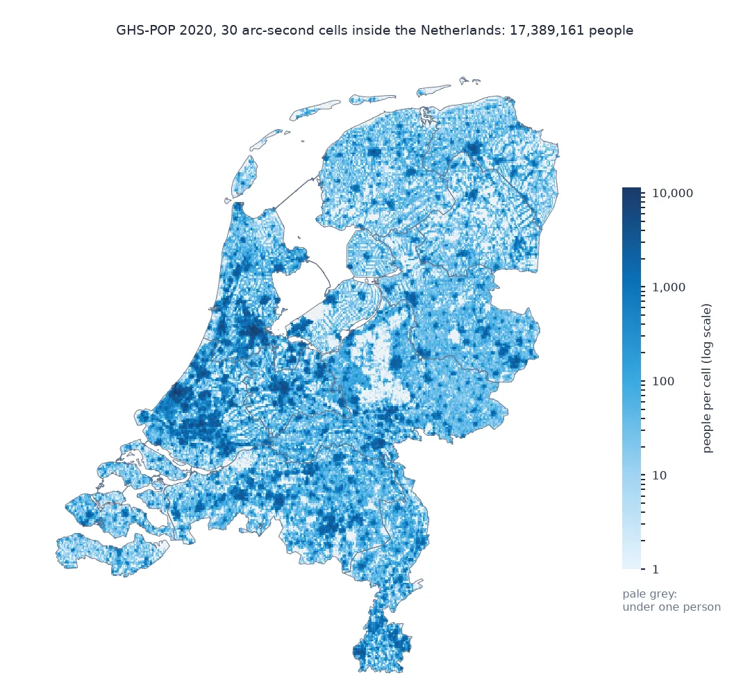
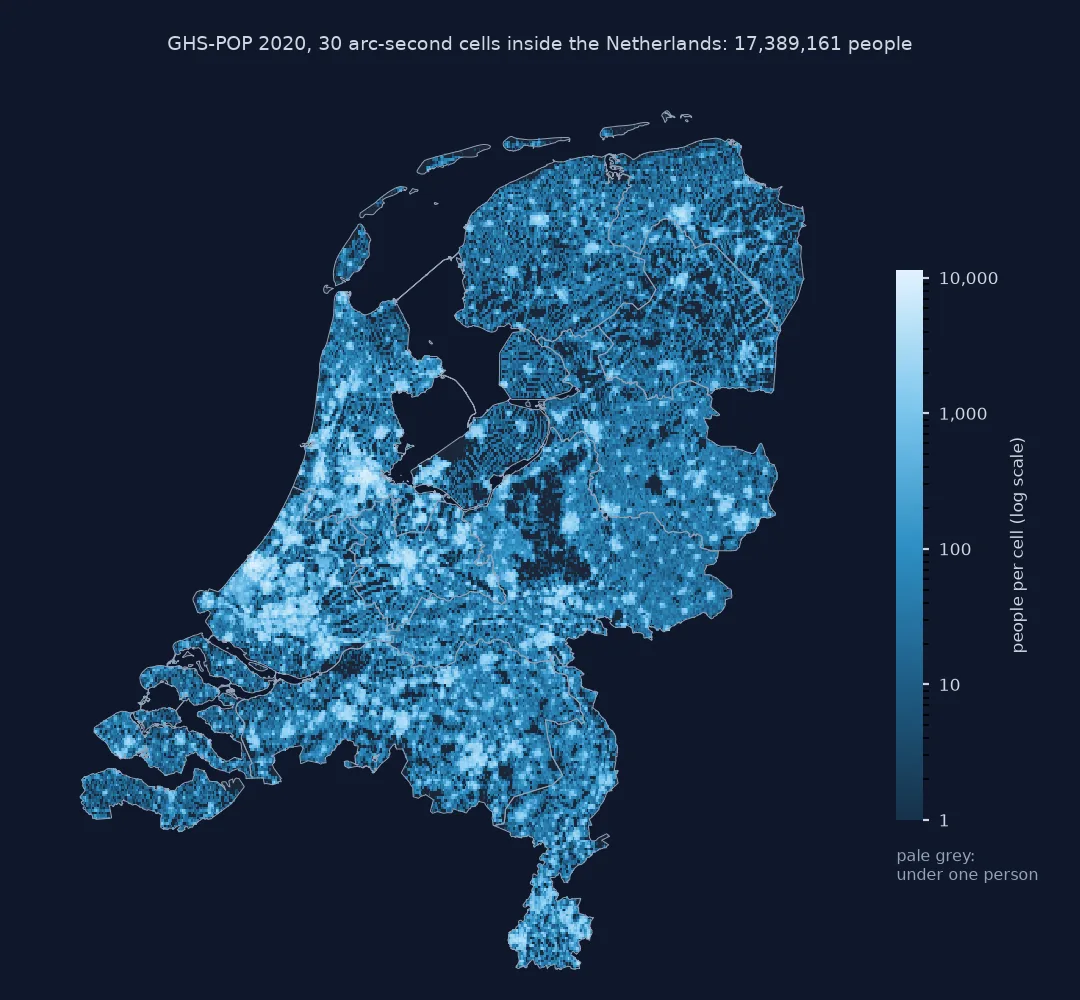
Find the tile, clip without changing the total, measure concentration
1. Find the tile and read its grid
GHSL cuts each global layer into tiles named by row and column, R4_C19 for the one with the Netherlands. The tile's metadata says what one cell is:
with rasterio.open(TILE) as src:
    print(f"{TILE.name}\n{src.width} x {src.height} cells, {src.res[0] * 3600:.0f} arc-seconds, {src.crs}, {src.dtypes[0]}, nodata {src.nodata}")
    print(f"bounds: {src.bounds.left:.1f} to {src.bounds.right:.1f} E, {src.bounds.bottom:.1f} to {src.bounds.top:.1f} N")
    whole = src.read(1, masked=True)
print(f"people in the whole tile: {whole.sum():,.0f}; largest cell {whole.max():,.0f}")
GHS_POP_E2020_GLOBE_R2023A_4326_30ss_V1_0_R4_C19.tif
1200 x 1200 cells, 30 arc-seconds, EPSG:4326, float64, nodata None
bounds: -0.0 to 10.0 E, 49.1 to 59.1 N
people in the whole tile: 91,471,436; largest cell 16,403
The tile is 1,200 by 1,200 cells of 30 arc-seconds, stored as 64-bit floats in WGS 84 with no nodata value declared, so the sea is simply zero. It runs from 0° to 10°E and 49.1°N to 59.1°N, holds 91.5 million people, and its fullest cell 16,403.
2. Clip without changing the total
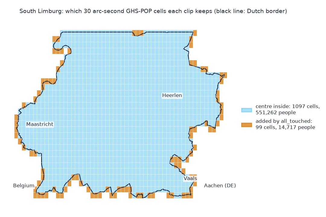
mask keeps a cell when its centre falls inside the boundary. With all_touched=True it keeps every cell the boundary touches, which adds the border cells shared with Belgium, Germany and the sea:
def clipped_total(**kw):
    with rasterio.open(TILE) as src:
        a, _ = mask(src, NL.to_crs(src.crs).geometry, crop=True, filled=False, **kw)
    return a.sum(), a.count()
for label, kw in (("cell centre inside", {}), ("all touched", {"all_touched": True})):
    total, cells = clipped_total(**kw)
    print(f"{label:>18}: {total:,.0f} people, {cells:,} cells, {total / OFFICIAL - 1:+.2%} against the official count")
cell centre inside: 17,389,161 people, 66,493 cells, -0.11% against the official count
all touched: 17,494,194 people, 69,267 cells, +0.50% against the official count
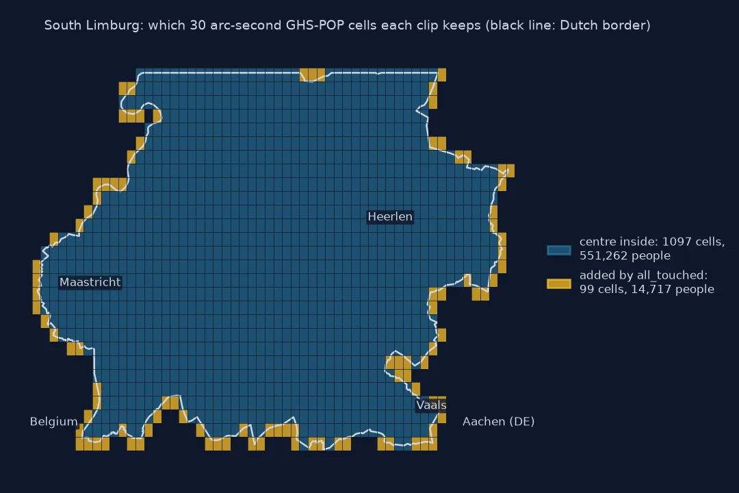
Counting by cell centre gives the total above. Counting every touched cell adds 2,774 border cells and 105,033 people, turning a 0.11% shortfall into a 0.50% overcount: those cells straddle the border with Belgium and Germany or the coast, and only part of each lies inside.
3. How concentrated the population is
Sort the cells from densest to emptiest and ask how few hold most people:
v = np.sort(grid.compressed())[::-1]
share = np.cumsum(v) / v.sum()
for q in (0.5, 0.8):
    n = int(np.searchsorted(share, q)) + 1
    print(f"{q:.0%} of people live in the densest {n:,} cells, {n / v.size:.1%} of the land cells")
print(f"cells with fewer than one person: {(v < 1).sum():,} ({(v < 1).mean():.1%})")
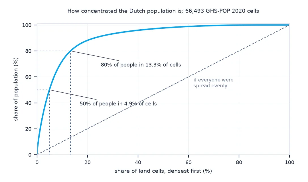
50% of people live in the densest 3,270 cells, 4.9% of the land cells
80% of people live in the densest 8,844 cells, 13.3% of the land cells
cells with fewer than one person: 8,215 (12.4%)
Half the population lives in 3,270 cells, 4.9% of the land cells, and 80% in 13.3% of them. At the other end, 8,215 cells, one in eight, hold less than one person each: the model spreading a census unit's people thinly over its sparsely built cells.
Writing the clipped grid to a GeoTIFF
The data used on this page
The GHS-POP R2023A epoch 2020 grid at 30 arc-seconds in WGS 84 from the JRC's open data server, the 2020 boundary of the Netherlands from the PDOK CBS gebiedsindelingen web feature service, and the population on 1 January 2020 from Statistics Netherlands' StatLine table 03759ned.
import io
import json
import zipfile
from pathlib import Path

import geopandas as gpd
import numpy as np
import rasterio
import requests
from rasterio.mask import mask

Path("data").mkdir(exist_ok=True)
GHSL = "https://jeodpp.jrc.ec.europa.eu/ftp/jrc-opendata/GHSL"
name = "GHS_POP_E2020_GLOBE_R2023A_4326_30ss"
TILE = Path("data", f"{name}_V1_0_R4_C19.tif")
if not TILE.exists():
    url = f"{GHSL}/GHS_POP_GLOBE_R2023A/{name}/V1-0/tiles/{TILE.stem}.zip"
    zipfile.ZipFile(io.BytesIO(requests.get(url, timeout=600).content)).extract(TILE.name, "data")
B = Path("data/landsdeel_2020.geojson")                                # the four parts of the country, land only
if not B.exists():
    B.write_bytes(requests.get("https://service.pdok.nl/cbs/gebiedsindelingen/2020/wfs/v1_0", timeout=300, params={
        "service": "WFS", "version": "2.0.0", "request": "GetFeature", "typeName": "gebiedsindelingen:landsdeel_gegeneraliseerd",
        "outputFormat": "application/json", "srsName": "EPSG:28992"}).content)
NL = gpd.read_file(B).dissolve()
C = Path("data/cbs_pop_2020.json")
if not C.exists():
    C.write_bytes(requests.get("https://opendata.cbs.nl/ODataApi/odata/03759ned/TypedDataSet", timeout=300, params={
        "$filter": "Geslacht eq 'T001038' and Leeftijd eq '10000' and BurgerlijkeStaat eq 'T001019' and Perioden eq '2020JJ00' "
                   "and (substring(RegioS,0,2) eq 'GM' or substring(RegioS,0,2) eq 'NL')",
        "$select": "RegioS,BevolkingOp1Januari_1"}).content)
OFFICIAL = next(r["BevolkingOp1Januari_1"] for r in json.loads(C.read_text())["value"] if r["RegioS"].startswith("NL"))
print(f"tile {TILE.stat().st_size / 1e6:.1f} MB; boundary {NL.area.sum() / 1e6:,.0f} km2 of land; official population {OFFICIAL:,}")
tile 4.3 MB; boundary 35,085 km2 of land; official population 17,407,585
The tile is 4.3 MB. The boundary covers 35,085 km² of land, without the IJsselmeer, the Wadden Sea and coastal waters.
Example 1: write the clipped grid to a GeoTIFF
The masked array and the transform mask returns are all a new file needs, plus a nodata value. Step 1 showed that the 30 arc-second tile declares none, and a masked array filled without one writes its default fill value, 1e20, into every cell outside the boundary. Set one explicitly; GHSL's Mollweide layers use -200:
with rasterio.open(TILE) as src:
    profile = src.profile | {"height": grid.shape[1], "width": grid.shape[2], "transform": transform,
                             "compress": "deflate", "nodata": -200}
with rasterio.open("ghs_pop_2020_nl.tif", "w", **profile) as dst:
    dst.write(grid.filled(-200))
with rasterio.open("ghs_pop_2020_nl.tif") as check:
    back = check.read(1, masked=True)
    print(f"{check.width} x {check.height} cells; total read back {back.sum():,.0f}; file {Path('ghs_pop_2020_nl.tif').stat().st_size / 1e3:,.0f} kB")
466 x 337 cells; total read back 17,389,161; file 444 kB
The clipped file is 466 by 337 cells, 444 kB with deflate compression, and reads back to exactly the clipped total.
GHS-POP is a model, not a count
GHS-POP is a model, not a count. The JRC starts from census or register populations for administrative units, collected through CIESIN's Gridded Population of the World, and spreads each unit's people over its cells in proportion to the residential built-up volume mapped from satellite imagery in the same GHSL release. A cell with more residential volume gets more people, and a cell with none gets few or none. The input metadata spreadsheet lists the inputs per country: for the Netherlands, Statistics Netherlands' 2011 population register for 418 municipalities, with growth rates from 2001 to 2011. The 2020 epoch is therefore a projection from 2011 municipal counts, distributed over 2020 buildings, not a 2020 count.
That is why the national total here lands within 0.11% of the register, which the model started from, and why the values are fractions of people: a cell with 0.3 people is a statement about density, not a person.
Tiles, two CRSs and epochs
- Tiles and the global file: the 30 arc-second layer is also published as one global file; a tile is smaller and faster when the area fits in one. An area across a tile edge needs a mosaic first (
rasterio.merge.merge). - Two CRSs: every GHS-POP epoch exists in WGS 84 (3 and 30 arc-seconds) and in World Mollweide (100 m and 1 km). The Mollweide cells are equal-area; the WGS 84 cells shrink towards the poles.
- Epoch is not year: E2020 is the 2020 epoch of the R2023A release; a later release revises earlier epochs as well.
- Coastlines: the PDOK boundaries used here are land only, so coastal and IJsselmeer cells whose centres fall in water are left out.
Internal links
- How to delineate an urban extent from GHSL in Python — the same grid, clustered into urban centres
- How to compute population-weighted exposure in Python — GHS-POP as weights
- Zonal statistics in Python — summing a raster by polygons
FAQ
How do I download GHSL population data in Python?
Build the tile URL from the JRC open data server's folder for the epoch and grid, download the zip with requests, extract the GeoTIFF with zipfile, and open it with rasterio.
Which GHSL tile covers the Netherlands?
In the 30 arc-second WGS 84 layer, the whole country is in tile R4_C19, which covers 0° to 10°E and 49.1°N to 59.1°N.
Is GHSL population accurate?
For the Netherlands in 2020, the clipped total on this page comes within a fraction of a percent of the official count; for small areas the errors are larger, because the model spreads census totals over built-up areas.
Should I use all_touched when clipping a population raster?
No, not for totals: it keeps every cell the boundary touches and adds people from across the border, as step 2 shows. Use cell centres, or fractional coverage for small areas.