How to Build Rainfall IDF Curves in Python from a Gauge Record

Problem statement

Intensity-duration-frequency (IDF) curves answer the design question behind every culvert, storm drain and detention pond: how hard does it rain, for how long, how often? Building them from a gauge looks simple: annual maxima for each duration, a distribution fit, and read-off. But a real hourly record has flagged values, multi-hour accumulations, decades with gaps, and clock-hour totals that miss the true peak hour. Each one moves the curve, and some move it a long way.

This page builds IDF curves for Conroe, Texas, north of Houston, from the NCEI Hourly Precipitation Data record (1947–2026). It compares them with NOAA Atlas 14, the official US values, and places Hurricane Beryl (2024), Hurricane Harvey (2017) and the October 1994 flood on the curves.

Quick answer

Clean the hourly series, take annual maxima of sliding sums for each duration from years complete enough to trust, fit a GEV per duration, and compare with Atlas 14:

rows = []
for D in DURATIONS:
    am = annual_max(D)
    shape, loc, scale = genextreme.fit(am, -0.1, loc=np.median(am), scale=am.std() / 2)
    rows.append({"duration_h": D, "years": len(am), **{f"{T}-yr": genextreme.ppf(1 - 1 / T, shape, loc, scale) for T in (2, 10, 100)},
                 **{f"A14 {T}-yr": ATLAS14.loc[D, T] for T in (2, 10, 100)}})
IDF = pd.DataFrame(rows).set_index("duration_h")
print(IDF.round(0).astype(int).to_string())

            years  2-yr  10-yr  100-yr  A14 2-yr  A14 10-yr  A14 100-yr
duration_h                                                             
1              57    47     70      95        50         78         118
2              57    62     97     147        62        103         172
3              59    69    113     197        69        120         212
6              58    83    143     284        81        148         282
12             56    98    173     322        93        176         345
24             55   108    195     364       106        204         409

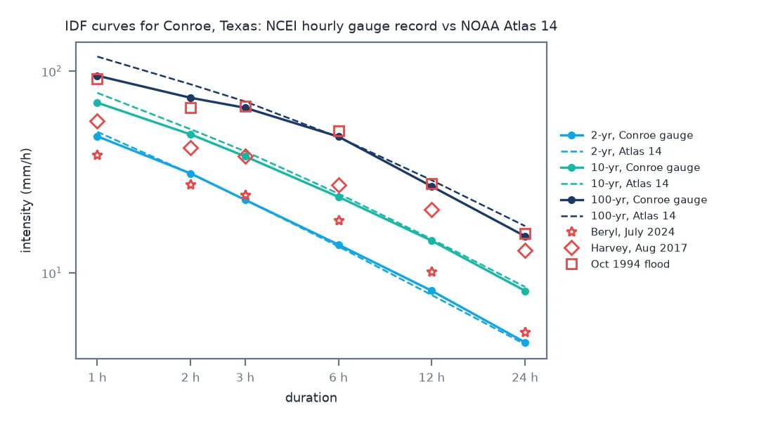
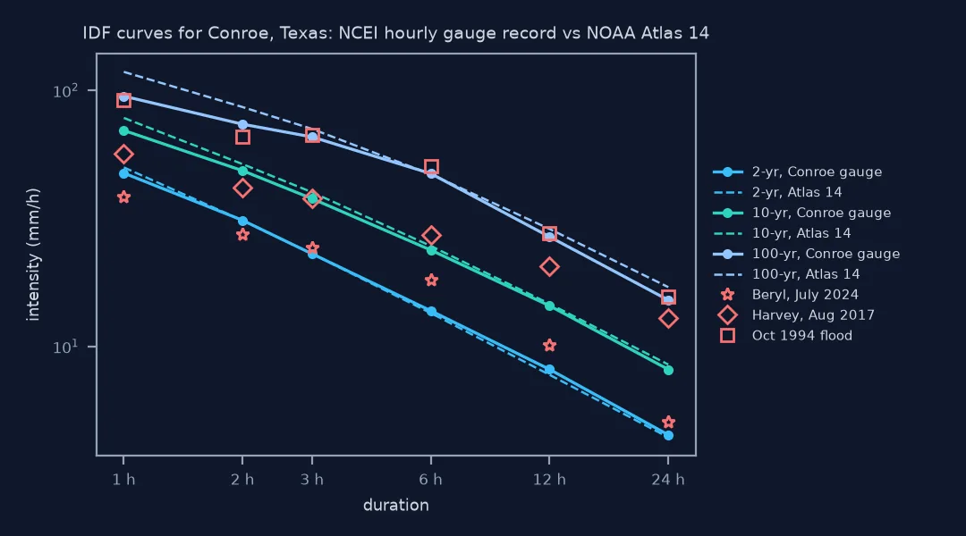
Clean the record, trust the right years, sliding maxima, a fit

1. Clean the hourly record

HPD stores hundredths of an inch, one row per day with 24 hourly values, each with a measurement flag and a quality flag. Treat −9999 as missing; drop values that failed quality control; and drop multi-hour accumulations (flags a, ., A), whose total cannot be placed in a single hour:

qf_counts = pd.Series(QF.ravel()).value_counts()
mf_counts = pd.Series(MF.ravel()).value_counts()
print("quality flags:", qf_counts.drop("", errors="ignore").to_dict())
print("accumulation flags:", {k: int(mf_counts.get(k, 0)) for k in ("a", ".", "A")}, "| missing (-9999):", int((VAL < 0).sum()))
print(f"{len(rain):,} hours from {rain.index.min():%Y-%m-%d} to {rain.index.max():%Y-%m-%d}; {rain.notna().mean():.1%} usable")

quality flags: {'M': 3679, 'D': 1310, 'A': 169, 'R': 102, 'q': 47, 'G': 2}
accumulation flags: {'a': 165, '.': 1609, 'A': 169} | missing (-9999): 8310
694,032 hours from 1947-07-01 to 2026-09-01; 83.8% usable

2. Decide which years to trust

An annual maximum from a year with half its hours missing may simply have missed the storm. The usual rule keeps years with at least 90% of hours:

share = rain.notna().groupby(rain.index.year).mean()
print(f"{(share >= 0.9).sum()} of {len(share)} years are at least 90% complete")
print("2017 (Harvey):", f"{share[2017]:.1%}", "| 2024 (Beryl):", f"{share[2024]:.1%}")

39 of 80 years are at least 90% complete
2017 (Harvey): 79.8% | 2024 (Beryl): 79.5%

The 90% rule throws out both hurricane years, and most of the 2010s. But a missing hour can only make a year's true maximum larger, never smaller. So a year whose observed maximum already exceeds the median of the complete years carries real information and is kept. That is the rule annual_max applies:

for D in (1, 24):
    strict = annual_max(D, rule="strict")
    kept = annual_max(D)
    print(f"{D:2d} h: {len(strict)} years under the 90% rule, {len(kept)} with large incomplete years added; "
          f"added include 2017: {2017 in kept.index and 2017 not in strict.index}, 2024: {2024 in kept.index and 2024 not in strict.index}")

 1 h: 39 years under the 90% rule, 57 with large incomplete years added; added include 2017: True, 2024: True
24 h: 39 years under the 90% rule, 55 with large incomplete years added; added include 2017: True, 2024: True

3. Take sliding, not calendar, maxima

A 24-hour maximum is the largest sum of any 24 consecutive hours, not the wettest calendar day; storms do not respect midnight:

r24 = rain.rolling(24, min_periods=24).sum()
day = rain.resample("D").sum(min_count=24)
top = annual_max(24).sort_values(ascending=False).head(5)
print(pd.DataFrame({"sliding 24 h": top, "wettest calendar day": [day[str(y)].max() for y in top.index],
                    "ending": [r24[str(y)].idxmax().strftime("%Y-%m-%d %H:00") for y in top.index]}).round(1).to_string())

      sliding 24 h  wettest calendar day            ending
1994         375.9                 142.2  1994-10-17 05:00
2017         310.6                 272.5  2017-08-27 14:00
2001         264.2                 259.1  2001-06-08 20:00
1961         253.5                 175.5  1961-09-12 04:00
1979         190.5                 119.4  1979-04-19 10:00

The October 1994 flood, not Harvey, holds this gauge's 24-hour record. The wettest calendar day is lower for every storm: by 2% in June 2001, by 12% for Harvey, and by much more in 1994 and 1961, whose storms ran across midnight. October 1994 also shows why completeness matters: only six hours of 17 October were recorded, and they held 233.7 mm, so that day has no complete calendar total at all.

4. Fit and read the curves

The quick answer fits a generalised extreme value (GEV) distribution to each duration's annual maxima. Convert depths to intensities to draw the classic IDF diagram:

intensity = IDF[[f"{T}-yr" for T in (2, 10, 100)]].div(IDF.index.to_series(), axis=0)
print(intensity.round(1).to_string())
print(f"100-yr / 2-yr depth ratio: 1 h {IDF.loc[1, '100-yr'] / IDF.loc[1, '2-yr']:.1f}, 24 h {IDF.loc[24, '100-yr'] / IDF.loc[24, '2-yr']:.1f}")

            2-yr  10-yr  100-yr
duration_h                     
1           47.5   69.7    94.8
2           31.1   48.6    73.7
3           23.0   37.8    65.8
6           13.8   23.8    47.3
12           8.1   14.4    26.8
24           4.5    8.1    15.2
100-yr / 2-yr depth ratio: 1 h 2.0, 24 h 3.4

The spread between frequent and rare storms widens with duration here: long, slow-moving tropical systems make the 24-hour tail heavy.

5. Check against Atlas 14

At 2 and 10 years, and at 6 hours for every return period, the gauge-only curves land within a few percent of Atlas 14. The 1-hour curve falls short by 6% at 2 years and 20% at 100 years, and the 24-hour 100-year value by 11%. There are two reasons. The record counts clock hours (00:00–01:00, 01:00–02:00), and the heaviest 60 minutes usually straddle two of them, so a clock-hour maximum is systematically below the true 60-minute maximum. Atlas 14 converts clock-hour maxima to true maxima. It also pools many stations in a region, so its estimates do not hang on one gauge's few extreme years.

How rare Beryl and Harvey were at Conroe

The data used on this page

NCEI Hourly Precipitation Data v2, station USC00411956 (Conroe, TX, a Fischer–Porter weighing gauge); NOAA Atlas 14 Volume 11 annual-maximum-series depths for the same coordinates, from the Precipitation Frequency Data Server.

import re
from pathlib import Path

import numpy as np
import pandas as pd
import requests
from scipy.stats import genextreme

Path("data").mkdir(exist_ok=True)
HPD = Path("data/USC00411956.csv")
if not HPD.exists():
    HPD.write_bytes(requests.get("https://www.ncei.noaa.gov/data/coop-hourly-precipitation/v2/access/USC00411956.csv", timeout=600).content)
raw = pd.read_csv(HPD, dtype=str)
VAL = raw[[f"HR{h:02d}Val" for h in range(24)]].astype(float).values
QF = np.char.strip(raw[[f"HR{h:02d}QF" for h in range(24)]].fillna("").values.astype(str))
MF = np.char.strip(raw[[f"HR{h:02d}MF" for h in range(24)]].fillna("").values.astype(str))
bad = (VAL < 0) | (QF != "") | np.isin(MF, ["a", ".", "A"])
stamps = pd.to_datetime(raw.DATE).values[:, None] + np.arange(24) * np.timedelta64(1, "h")
rain = pd.Series(np.where(bad, np.nan, VAL * 0.254).ravel(), index=pd.DatetimeIndex(stamps.ravel())).sort_index()
rain = rain[~rain.index.duplicated()].asfreq("h")                     # mm per clock hour, local standard time
DURATIONS = (1, 2, 3, 6, 12, 24)


def annual_max(D, rule="kept"):
    share = rain.notna().groupby(rain.index.year).mean()
    sums = rain.rolling(D, min_periods=D).sum()
    am = sums.groupby(sums.index.year).max()
    keep = share >= 0.9
    if rule == "kept":
        keep |= (share >= 0.5) & (am > am[share >= 0.9].median())
    return am[keep].dropna()


pfds = requests.get("https://hdsc.nws.noaa.gov/cgi-bin/new/cgi_readH5.py", timeout=120, params={
    "lat": 30.3302, "lon": -95.4831, "type": "pf", "data": "depth", "units": "metric", "series": "ams"}).text
q = np.array(eval(re.search(r"quantiles = (\[\[.*?\]\]);", pfds, re.S).group(1)), float)
ATLAS14 = pd.DataFrame(q[4:10][:, [0, 2, 5]], index=list(DURATIONS), columns=[2, 10, 100])    # rows 60 min .. 24 h
print(f"HPD: {len(raw):,} days; Atlas 14 AMS depths for {len(ATLAS14)} durations, mm")

HPD: 24,594 days; Atlas 14 AMS depths for 6 durations, mm

Example 1: how rare were Beryl and Harvey at Conroe?

def ari(depth, D):
    p = genextreme.sf(depth, *genextreme.fit(annual_max(D), -0.1, loc=np.median(annual_max(D)), scale=annual_max(D).std() / 2))
    return 1 / p

for name, (a, b) in {"Beryl 2024": ("2024-07-07", "2024-07-10"), "Harvey 2017": ("2017-08-25", "2017-08-31"),
                     "October 1994": ("1994-10-15", "1994-10-20")}.items():
    w = rain[a:b]
    peaks = {D: w.rolling(D, min_periods=D).sum().max() for D in (1, 6, 24)}
    print(f"{name:13s} " + "  ".join(f"{D:2d} h {v:5.1f} mm (~{ari(v, D):,.0f} yr)" for D, v in peaks.items())
          + f"  | {int(w.isna().sum())} hours missing")

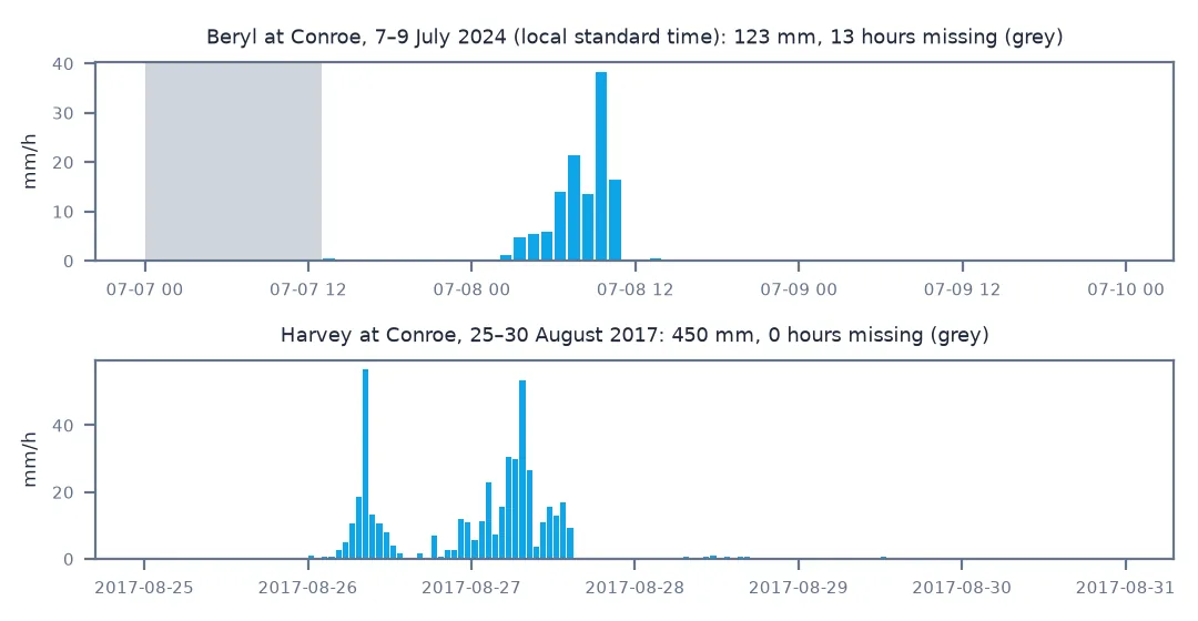
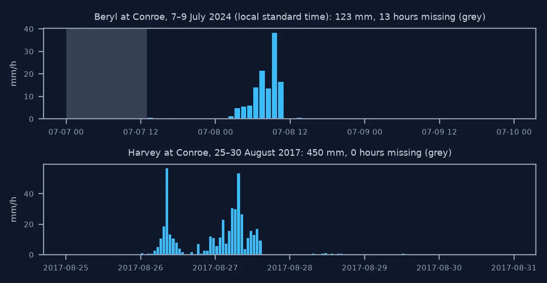
Beryl 2024     1 h  38.4 mm (~1 yr)   6 h 109.5 mm (~4 yr)  24 h 122.2 mm (~3 yr)  | 13 hours missing
Harvey 2017    1 h  56.6 mm (~4 yr)   6 h 163.3 mm (~16 yr)  24 h 310.6 mm (~54 yr)  | 0 hours missing
October 1994   1 h  91.4 mm (~72 yr)   6 h 302.3 mm (~124 yr)  24 h 375.9 mm (~114 yr)  | 29 hours missing

At Conroe, Beryl was an ordinary storm of the kind expected every three or four years — its worst rain fell south, over Houston. Harvey's 24 hours rank about 1-in-50 here. The October 1994 flood exceeds 100 years at 6 and 24 hours, and even its total is a lower bound, with 29 hours missing.

Example 2: what the completeness rule does to the 100-year value

for D in (1, 6, 24):
    out = []
    for rule in ("strict", "kept"):
        am = annual_max(D, rule)
        out.append(genextreme.ppf(0.99, *genextreme.fit(am, -0.1, loc=np.median(am), scale=am.std() / 2)))
    print(f"{D:2d} h 100-yr: {out[0]:5.0f} mm (90% rule) -> {out[1]:5.0f} mm (large incomplete years kept); Atlas 14 {ATLAS14.loc[D, 100]:.0f} mm")

 1 h 100-yr:   101 mm (90% rule) ->    95 mm (large incomplete years kept); Atlas 14 118 mm
 6 h 100-yr:   241 mm (90% rule) ->   284 mm (large incomplete years kept); Atlas 14 282 mm
24 h 100-yr:   328 mm (90% rule) ->   364 mm (large incomplete years kept); Atlas 14 409 mm

At 6 and 24 hours, throwing away incomplete years removes the years when the gauge recorded floods and lowers the 100-year estimate by 15% and 10%. At 1 hour the strict rule comes out slightly higher, because the years it drops were not extreme for one-hour bursts. A completeness rule is not neutral. Check what it removes.

What an IDF curve summarises

An IDF curve summarises the extreme-value distribution of rainfall depth at a set of durations. For each duration, the annual maximum series is fitted with a GEV. The return level for T years is the depth exceeded with probability 1/T in any year. Dividing by the duration gives intensity, and plotting intensity against duration on log axes gives the familiar falling curves, one per return period.

The arithmetic is quick. The judgement is in the data. Which values are real hourly totals? Which years can be trusted? Are the maxima sliding or fixed? Is one gauge enough? For Conroe, a careful single-gauge analysis gets close to Atlas 14 at 6–24 hours and falls short at 1 hour, for reasons that are understood. The official curves should still be the default for design. A local analysis like this one is how you check them, extend them to a new duration, or see how a recent storm changes the picture.

Clock-hour data, local time and fit starting points

• Clock-hour data understate short durations; Atlas 14 applies conversion factors to reach true 60-minute and 24-hour maxima.
• Hours are local standard time in HPD; a storm total split at midnight depends on that.
• The GEV fit needs a starting point; scipy's default start can fail on heavy-tailed rainfall.
• Thirty to sixty years of record gives wide uncertainty at 100 years; bootstrap it before quoting a single number.
• Non-stationarity: Atlas 14 assumes a stable climate; newer studies adjust for trends.
• Partial-duration series (all peaks above a threshold) give slightly different values from annual maxima at short return periods.

Internal links

• Rainfall return periods explained — GEV and what "100-year" means
• Rainfall totals come out wrong — missing hours and windows
• How to analyse a rain gauge network — completeness across many gauges
• How to read MRMS rainfall in Python — MRMS ARI uses Atlas 14
• Hurricane tracks from IBTrACS — the storms on these curves

FAQ

What is an IDF curve?

A set of curves giving rainfall intensity against duration for several return periods, built from the annual maxima of rainfall at each duration.

How many years of data do I need for IDF curves?

At least 20–30 complete years for frequent return periods; estimates beyond the record length (e.g. 100-year from 50 years) carry wide uncertainty.

Why is my 1-hour IDF value lower than NOAA Atlas 14?

Clock-hour data miss the true peak 60 minutes, and Atlas 14 pools regional stations. At Conroe the single-gauge 1-hour values are 6% lower at 2 years and 20% lower at 100 years.

Should I drop incomplete years from an annual maximum series?

Not automatically. A year with gaps whose observed maximum is already large carries real information — the true maximum can only be larger.