
How to Find Disease Clusters With a Spatial Scan Statistic in Python
On this page
Problem statement
A map of disease rates invites the eye to find clusters, and the eye finds them whether they are there or not. The spatial scan statistic, introduced by Martin Kulldorff in 1997, turns the question into a test: it moves a circular window over the map at every location and size, finds the window where cases most exceed what the population predicts, and asks how often a window that extreme would appear by chance. It is the method behind SaTScan, the standard tool for disease cluster detection, and its Poisson version needs only case counts and populations by area.
This page implements the Poisson scan statistic in NumPy and runs it on Lyme disease cases in Virginia's counties and independent cities for 2017–2021: 4,847 cases, against 1,100 in 2001–2005.
Quick answer
For each area, grow a circle through its nearest neighbours up to half the population, score every circle by its likelihood ratio, and keep the best:
def scan(cases, pop, order, max_share=0.5):
    """Kulldorff's Poisson scan: returns (log-likelihood ratio, centre index, number of areas in the circle)."""
    C, P = cases.sum(), pop.sum()
    best = (0.0, None, None)
    for i in range(len(pop)):
        cp, cc = np.cumsum(pop[order[i]]), np.cumsum(cases[order[i]])        # circle grows one neighbour at a time
        k = np.searchsorted(cp, max_share * P, side="right")
        if k == 0:                                                           # the centre alone is over the limit
            continue
        cp, cc = cp[:k], cc[:k]
        E = C * cp / P                                                       # expected cases in the circle
        with np.errstate(divide="ignore", invalid="ignore"):
            llr = np.where(cc > E, cc * np.log(cc / E) + (C - cc) * np.log((C - cc) / (C - E)), 0.0)
        j = int(np.nanargmax(llr))
        if llr[j] > best[0]:
            best = (float(llr[j]), i, j + 1)
    return best

llr, centre, size = scan(CASES, POP, ORDER)
members = ORDER[centre][:size]
obs, exp = CASES[members].sum(), CASES.sum() * POP[members].sum() / POP.sum()
print(f"most likely cluster: {size} areas around {D.NAMELSAD.iloc[centre]}; {obs:.0f} cases against {exp:.0f} expected; LLR {llr:.1f}")
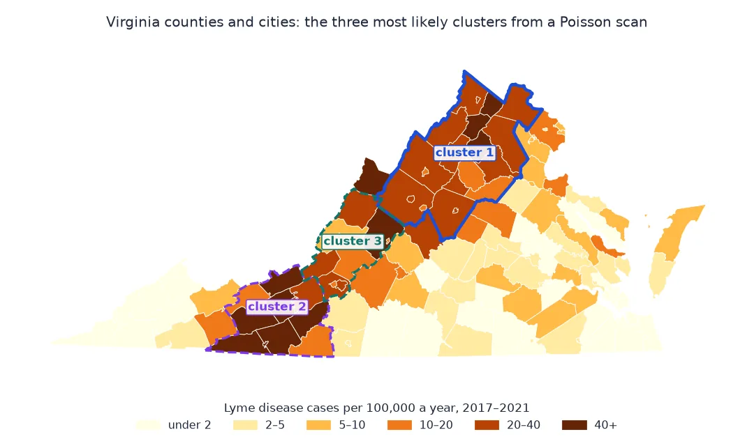
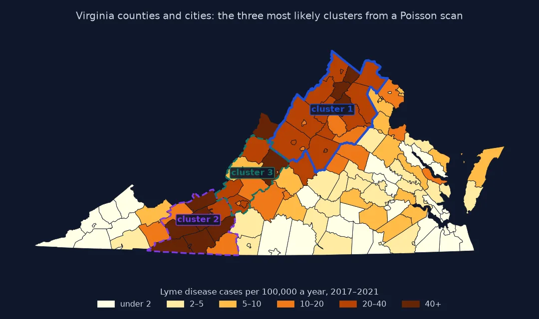
most likely cluster: 20 areas around Shenandoah County; 2017 cases against 723 expected; LLR 1003.9
Candidate windows, a Monte Carlo test, relative risk
1. Build the candidate windows
Each window is a centre and the areas nearest to it. Sorting every area's neighbours by distance once makes each circle a prefix of a sorted list:
print(f"{len(D)} areas; candidate circles: up to {len(D)} centres × the neighbours within half the population")
n_windows = sum(np.searchsorted(np.cumsum(POP[ORDER[i]]), 0.5 * POP.sum(), side="right") for i in range(len(D)))
print(f"{n_windows:,} circles scored in one scan")
133 areas; candidate circles: up to 133 centres × the neighbours within half the population
9,400 circles scored in one scan
2. Test the cluster by Monte Carlo
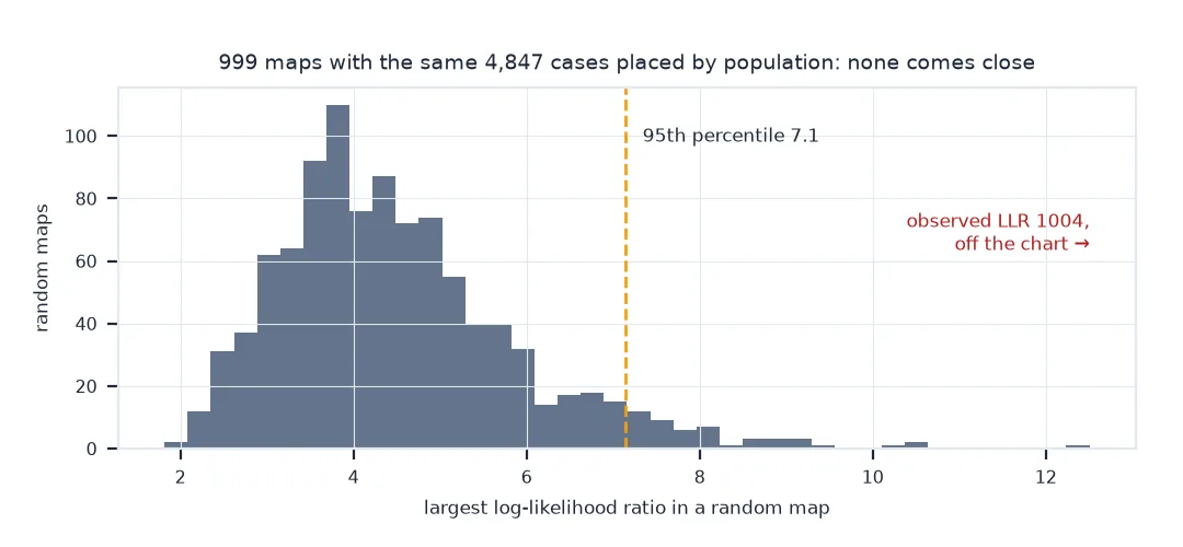
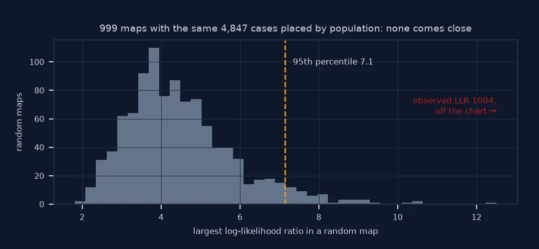
The likelihood ratio of the best circle has no simple distribution, because it is the maximum over thousands of overlapping windows. Kulldorff's solution is to redistribute the same number of cases at random in proportion to population, scan each random map the same way, and see where the real maximum ranks:
rng = np.random.default_rng(1)
sims = np.array([scan(rng.multinomial(int(CASES.sum()), POP / POP.sum()), POP, ORDER)[0] for _ in range(999)])
p = (1 + (sims >= llr).sum()) / (len(sims) + 1)
print(f"largest LLR in 999 random maps: {sims.max():.1f} (95th percentile {np.percentile(sims, 95):.1f}); observed {llr:.1f}; p = {p:.3f}")
largest LLR in 999 random maps: 12.5 (95th percentile 7.1); observed 1003.9; p = 0.001
With 999 replications the smallest possible p-value is 0.001, so a result of 0.001 means "more extreme than every random map", not an exact probability.
3. Report the cluster as a relative risk
inside_rate = obs / POP[members].sum()
outside_rate = (CASES.sum() - obs) / (POP.sum() - POP[members].sum())
print(f"relative risk inside against outside: {inside_rate / outside_rate:.2f}; "
      f"{inside_rate * 1e5:.1f} against {outside_rate * 1e5:.1f} cases per 100,000 a year")                # POP is person-years
print("areas:", ", ".join(D.NAMELSAD.iloc[members].str.replace(" County", "")))
relative risk inside against outside: 4.07; 31.3 against 7.7 cases per 100,000 a year
areas: Shenandoah, Page, Warren, Rappahannock, Rockingham, Frederick, Winchester city, Harrisonburg city, Madison, Clarke, Greene, Fauquier, Culpeper, Orange, Loudoun, Staunton city, Augusta, Charlottesville city, Waynesboro city, Albemarle
Secondary clusters and window size
The data used on this page
Lyme disease case counts by county from the CDC, 2001–2023, of which 2017–2021 are used here because the surveillance case definition changed in 2022; the Census Bureau's 2020 population estimates base by county; and the 2021 cartographic boundary file of counties. Virginia's independent cities are county equivalents and are treated as areas like the counties.
from pathlib import Path

import geopandas as gpd
import numpy as np
import pandas as pd
import requests

Path("data").mkdir(exist_ok=True)
SRC = {"LD_Case_Counts_by_County_2023.csv": "https://www.cdc.gov/lyme/media/files/2025/02/LD_Case_Counts_by_County_2023_updated.csv",
       "co-est2024-alldata.csv": "https://www2.census.gov/programs-surveys/popest/datasets/2020-2024/counties/totals/co-est2024-alldata.csv",
       "cb_2021_us_county_5m.zip": "https://www2.census.gov/geo/tiger/GENZ2021/shp/cb_2021_us_county_5m.zip"}
for name, url in SRC.items():
    if not Path("data", name).exists():
        Path("data", name).write_bytes(requests.get(url, timeout=300).content)

lyme = pd.read_csv("data/LD_Case_Counts_by_County_2023.csv", encoding="latin-1")      # not UTF-8
lyme["GEOID"] = lyme.stcode.astype(str).str.zfill(2) + lyme.ctycode.astype(str).str.zfill(3)
YEAR_COLS = ["Cases2017", "Cases2018", "Cases2019", "Cases2020", "cases2021"]          # the column case changes in 2021
YEARS = len(YEAR_COLS)
lyme["cases"] = lyme[YEAR_COLS].sum(axis=1)
va = lyme[lyme.stname == "Virginia"]
est = pd.read_csv("data/co-est2024-alldata.csv", encoding="latin-1", dtype={"STATE": str, "COUNTY": str}).query("SUMLEV == 50")
est["GEOID"] = est.STATE + est.COUNTY
D = (gpd.read_file("data/cb_2021_us_county_5m.zip").query("STATEFP == '51'").to_crs(3968)        # Virginia Lambert, metres
       .merge(va[["GEOID", "cases"]], on="GEOID").merge(est[["GEOID", "ESTIMATESBASE2020"]], on="GEOID"))
CASES = D.cases.to_numpy(float)
POP = D.ESTIMATESBASE2020.to_numpy(float) * YEARS                                       # person-years
xy = np.column_stack([D.centroid.x, D.centroid.y])
ORDER = np.argsort(np.linalg.norm(xy[:, None] - xy[None], axis=2), axis=1)
print(f"Virginia: {len(va)} areas in the Lyme file, {len(D)} matched to boundaries and population; "
      f"unmatched: {sorted(set(va.GEOID) - set(D.GEOID))}; {CASES.sum():,.0f} cases in {YEARS} years")
print(f"for comparison, 2001-2005: {va[['Cases2001', 'Cases2002', 'Cases2003', 'Cases2004', 'Cases2005']].sum().sum():,.0f} cases")
Virginia: 134 areas in the Lyme file, 133 matched to boundaries and population; unmatched: ['51515']; 4,847 cases in 5 years
for comparison, 2001-2005: 1,100 cases
Example 1: secondary clusters
Remove the areas of the most likely cluster and scan again, keeping only circles that do not overlap it. Secondary clusters are judged against the same Monte Carlo distribution, which makes their p-values conservative:
def scan_excluding(cases, pop, order, banned, max_share=0.5):
    keep = ~np.isin(np.arange(len(pop)), list(banned))
    best = (0.0, None, None)
    C, P = cases.sum(), pop.sum()
    for i in np.flatnonzero(keep):
        o = order[i]
        stop = np.argmax(~keep[o]) if (~keep[o]).any() else len(o)               # a circle may not reach into a found cluster
        cp, cc = np.cumsum(pop[o][:stop]), np.cumsum(cases[o][:stop])
        k = np.searchsorted(cp, max_share * P, side="right")
        E = C * cp[:k] / P
        with np.errstate(divide="ignore", invalid="ignore"):
            llr = np.where(cc[:k] > E, cc[:k] * np.log(cc[:k] / E) + (C - cc[:k]) * np.log((C - cc[:k]) / (C - E)), 0.0)
        if len(llr) and np.nanmax(llr) > best[0]:
            best = (float(np.nanmax(llr)), i, int(np.nanargmax(llr)) + 1)
    return best

banned = set(members)
for rank in (2, 3):
    l2, c2, s2 = scan_excluding(CASES, POP, ORDER, banned)
    m2 = ORDER[c2][:s2]
    e2 = CASES.sum() * POP[m2].sum() / POP.sum()
    print(f"cluster {rank}: {s2} areas around {D.NAMELSAD.iloc[c2]}; {CASES[m2].sum():.0f} cases against {e2:.0f}; "
          f"LLR {l2:.1f}; p {(1 + (sims >= l2).sum()) / 1000:.3f}")
    banned |= set(m2)
cluster 2: 11 areas around Carroll County; 879 cases against 160; LLR 835.9; p 0.001
cluster 3: 11 areas around Covington city; 325 cases against 181; LLR 48.4; p 0.001
The second cluster is in southwest Virginia, around Carroll County on the North Carolina border: 879 cases where the population predicts 160, a stronger excess than the first in relative terms, but in fewer people.
Example 2: the maximum window size
The 50% limit is SaTScan's default. Smaller limits find tighter clusters:
for share in (0.5, 0.25, 0.1):
    l, c, s = scan(CASES, POP, ORDER, max_share=share)
    m = ORDER[c][:s]
    print(f"max {share:.0%} of population: {s} areas, relative risk {CASES[m].sum() / POP[m].sum() / ((CASES.sum() - CASES[m].sum()) / (POP.sum() - POP[m].sum())):.2f}")
max 50% of population: 20 areas, relative risk 4.07
max 25% of population: 20 areas, relative risk 4.07
max 10% of population: 11 areas, relative risk 6.48
The first cluster holds less than a quarter of the state's population, so the 25% limit finds the same 20 areas; at 10% the scan keeps a tighter core of 11 with a relative risk of 6.48. Choose the limit before looking, and report it.
One hypothesis instead of many tests
The scan statistic avoids the multiple-testing problem of testing each area or each candidate cluster separately. It tests one hypothesis, that cases are distributed in proportion to population everywhere, against the alternative that there is some circle where the risk is higher. The test statistic is the maximum likelihood ratio over all circles, and the Monte Carlo replications include the same search, so the p-value already accounts for having looked everywhere.
What the scan finds is a circle, and real clusters are not circular. Here the most likely cluster is a band of counties along the Shenandoah Valley and the northern Piedmont, and the circle happens to fit it well: all 20 of its areas have higher rates than the rest of the state. A long, thin cluster in another place would be split into pieces or padded with low-rate neighbours, and elliptical windows and flexibly shaped scans exist for that reason. The Poisson model also assumes that, apart from the cluster, risk is proportional to population: with an infectious or environmental disease such as Lyme, whose risk depends on ticks and habitat, the "cluster" may be a whole region of higher risk rather than an outbreak.
Centroids, covariates and SaTScan
- Centroids: area centroids stand in for where people live; population-weighted centroids are better for large rural counties.
- Covariates: adjust expected counts for age or sex by computing them from age-specific rates, as in indirect standardisation.
- Case definitions: Lyme reporting changed in 2022; never scan across a change in definition.
- County changes: Bedford city (51515) merged into Bedford County in 2013 and has no boundary or population; it drops out.
- SaTScan: the free SaTScan software implements space-time, elliptical and other models; use it to check a home-made scan.
Internal links
- Disease clusters explained — why clusters appear by chance
- How to find hot spots with Getis-Ord Gi* — a local statistic for each area instead of one test
FAQ
What is the spatial scan statistic?
A cluster detection method that compares observed with expected cases in circular windows of every location and size and tests the most unusual one by Monte Carlo simulation.
Can I run a scan statistic in Python?
Yes. The Poisson version needs only counts, populations and coordinates, and fits in a few dozen lines of NumPy, as on this page.
What does the p-value of a scan statistic mean?
The share of random maps, with cases placed in proportion to population, whose most unusual window is at least as extreme as the observed one.
Why are scan statistic clusters circular?
Circles are the simplest family of windows that covers all locations and sizes; elliptical and irregular variants exist.