How to Map Age Groups from a Census Population Grid in Python

Problem statement

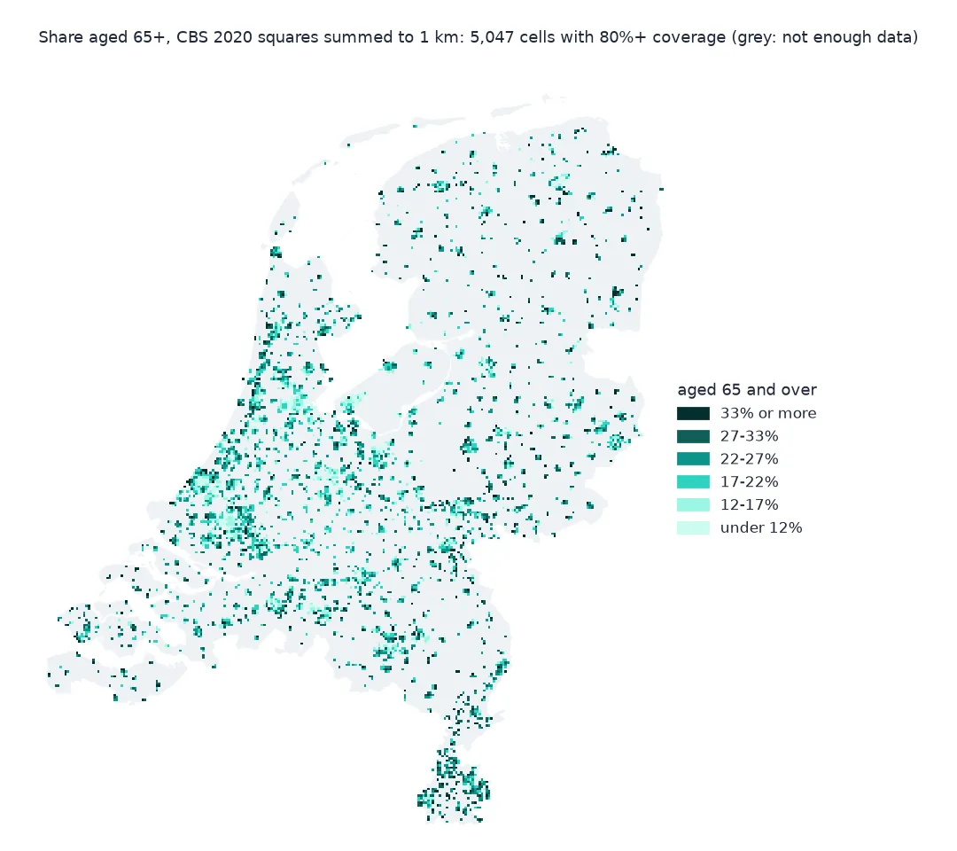
A census grid with age bands answers questions a total cannot: where the over-65s live, how far children are from schools, which neighbourhoods are ageing. The catch is confidentiality. Age bands split each square's residents into small groups, and small groups are suppressed far more often than totals, so a naive map of the share aged 65 and over is a map of where the data survived, and its sums fall well short of the official figures.

This page measures how much of each age band Statistics Netherlands' 2020 100 m grid publishes, recovers suppressed bands from the square totals where that is exact enough to use, aggregates to 1 km and to municipalities, and checks the result against the official age structure of every municipality.

Quick answer

Mask the suppression code, then compute shares only from squares where both the band and the total are published:

ok = (V.aantal_inwoners > 0) & (V.aantal_inwoners_65_jaar_en_ouder >= 0)
share = V.aantal_inwoners_65_jaar_en_ouder[ok].sum() / V.aantal_inwoners[ok].sum()
print(f"squares with the 65+ band published: {ok.sum():,} of {(V.aantal_inwoners > 0).sum():,}")
print(f"65+ share in those squares: {share:.1%}; official national share: {OFF_NL['k_65Tot80Jaar_8'] + OFF_NL['k_80JaarOfOuder_9']:,.0f} "
      f"of {OFF_NL['TotaleBevolking_1']:,.0f} = {(OFF_NL['k_65Tot80Jaar_8'] + OFF_NL['k_80JaarOfOuder_9']) / OFF_NL['TotaleBevolking_1']:.1%}")

squares with the 65+ band published: 204,332 of 379,905
65+ share in those squares: 22.6%; official national share: 3,392,555 of 17,407,585 = 19.5%

The 65+ band is published in 204,332 of the 379,905 squares with residents. In those squares, 22.6% of residents are 65 or over, against the official 19.5% for the country: the squares that survive suppression are older than the country.

How much of each band survives, recover bands, map the elderly share

1. How much of each band survives

For each band, count the squares where it is published and the residents of those squares:

pub = V[V.aantal_inwoners > 0]
for b in BANDS:
    p = pub[b] >= 0
    print(f"{b.replace('aantal_inwoners_', ''):>17}: published in {p.mean():.0%} of squares, which hold {pub.aantal_inwoners[p].sum() / pub.aantal_inwoners.sum():.0%} of residents; "
          f"band sum {pub[b][p].sum():,}")

    0_tot_15_jaar: published in 46% of squares, which hold 75% of residents; band sum 2,319,605
   15_tot_25_jaar: published in 39% of squares, which hold 69% of residents; band sum 1,680,455
   25_tot_45_jaar: published in 55% of squares, which hold 85% of residents; band sum 3,899,125
   45_tot_65_jaar: published in 68% of squares, which hold 91% of residents; band sum 4,311,375
 65_jaar_en_ouder: published in 54% of squares, which hold 77% of residents; band sum 2,919,025

Each band is published in 39% to 68% of the populated squares, which hold 69% to 91% of the residents. The youngest adults, 15 to 25, are suppressed most often. Summed, the published values account for 2.32 million children under 15 against 2.73 million officially, and 2.92 million over-65s against 3.39 million.

2. Recover a band from the total

The five bands add up to the square's total. Where exactly one band is suppressed, it can be recovered as the total minus the other four. Rounding to multiples of five makes the residual approximate, so check it where the band is known:

B = pub[BANDS]
missing = (B < 0).sum(axis=1)
print(f"squares with 0 bands suppressed: {(missing == 0).sum():,}; exactly 1: {(missing == 1).sum():,}; 2 or more: {(missing >= 2).sum():,}")
full = pub[missing == 0]
resid = full.aantal_inwoners - full[BANDS[:-1]].sum(axis=1)                      # pretend 65+ is missing
err = resid - full.aantal_inwoners_65_jaar_en_ouder
print(f"test on complete squares: residual 65+ within 5 of the published value in {(err.abs() <= 5).mean():.0%}, "
      f"mean error {err.mean():+.1f} people")
filled = B.where(B >= 0)
one = missing == 1
filled.loc[one] = filled.loc[one].apply(lambda r: r.fillna(pub.aantal_inwoners[r.name] - r.sum()).clip(lower=0), axis=1)
print(f"65+ after filling single gaps: {filled.aantal_inwoners_65_jaar_en_ouder.sum():,.0f} (published only: {pub.aantal_inwoners_65_jaar_en_ouder.clip(lower=0).sum():,})")

squares with 0 bands suppressed: 91,919; exactly 1: 65,377; 2 or more: 222,609
test on complete squares: residual 65+ within 5 of the published value in 99%, mean error +0.2 people
65+ after filling single gaps: 2,980,065 (published only: 2,919,025)

91,919 squares have all five bands and 65,377 have exactly one missing; the other 222,609 have two or more, and those cannot be separated. On the complete squares, the residual reproduces the published 65+ count within five people 99% of the time, with a mean error of +0.2, so it is safe to use. Filling single gaps adds 61,040 over-65s, a modest gain, because most suppressed bands sit in squares with several gaps.

3. Share aged 65 and over at 1 km

Aggregate the published-or-filled 65+ counts and the totals of the same squares to 1 km, and keep cells where those squares hold most of the residents:

k = pd.DataFrame({"kx": pub.x // 10, "ky": pub.y // 10, "total": pub.aantal_inwoners,
                  "old": filled.aantal_inwoners_65_jaar_en_ouder, "known": filled.aantal_inwoners_65_jaar_en_ouder.notna()})
K = k.groupby(["kx", "ky"]).apply(lambda g: pd.Series({"total": g.total.sum(), "old": g.old.sum(),
                                                         "coverage": g.total[g.known].sum() / g.total.sum(),
                                                         "share": g.old.sum() / g.total[g.known].sum() if g.known.any() else np.nan}), include_groups=False)
good = K[(K.coverage >= 0.8) & (K.total >= 100)]
print(f"1 km cells: {len(K):,}; with 80%+ coverage and 100+ residents: {len(good):,}, holding {good.total.sum() / K.total.sum():.0%} of residents")
print(f"65+ share across those cells: 10th percentile {good.share.quantile(0.1):.0%}, median {good.share.median():.0%}, 90th {good.share.quantile(0.9):.0%}")

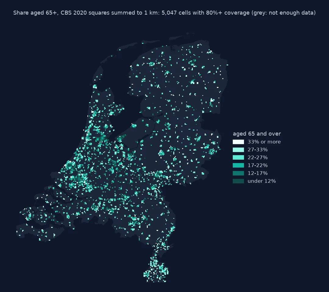
1 km cells: 23,556; with 80%+ coverage and 100+ residents: 5,047, holding 82% of residents
65+ share across those cells: 10th percentile 12%, median 22%, 90th 33%

5,047 of the 23,556 populated 1 km cells pass the coverage rule, and they hold 82% of all residents. Across them the share aged 65 and over runs from 12% at the 10th percentile to 33% at the 90th, around a median of 22%.

A check against the official age structure

The data used on this page

The CBS 100 m grid, final 2020 edition, the 2020 municipality boundaries from the PDOK CBS gebiedsindelingen web feature service, and the official age structure of every municipality on 1 January 2020 from Statistics Netherlands' regional key figures, StatLine table 70072ned.

import io
import json
import zipfile
from pathlib import Path

import geopandas as gpd
import numpy as np
import pandas as pd
import pyogrio
import requests

Path("data").mkdir(exist_ok=True)
GPKG = Path("data/cbs_vk100_2020_vol.gpkg")
if not GPKG.exists():
    url = "https://www.cbs.nl/-/media/cbs/dossiers/nederland-regionaal/vierkanten/100/2023-cbs_vk100_2020_vol.zip"
    zipfile.ZipFile(io.BytesIO(requests.get(url, timeout=900).content)).extract(GPKG.name, "data")
G = Path("data/gemeente_2020.geojson")
if not G.exists():
    G.write_bytes(requests.get("https://service.pdok.nl/cbs/gebiedsindelingen/2020/wfs/v1_0", timeout=300, params={
        "service": "WFS", "version": "2.0.0", "request": "GetFeature", "typeName": "gebiedsindelingen:gemeente_gegeneraliseerd",
        "outputFormat": "application/json", "srsName": "EPSG:28992"}).content)
A = Path("data/cbs_age_2020.json")
cols = "RegioS,TotaleBevolking_1,k_0Tot15Jaar_4,k_15Tot25Jaar_5,k_25Tot45Jaar_6,k_45Tot65Jaar_7,k_65Tot80Jaar_8,k_80JaarOfOuder_9"
if not A.exists():
    A.write_bytes(requests.get("https://opendata.cbs.nl/ODataApi/odata/70072ned/TypedDataSet", timeout=300, params={
        "$filter": "Perioden eq '2020JJ00' and (substring(RegioS,0,2) eq 'GM' or substring(RegioS,0,2) eq 'NL')", "$select": cols}).content)
AGE = pd.DataFrame(json.loads(A.read_text())["value"]).dropna()
AGE["RegioS"] = AGE.RegioS.str.strip()
OFF_NL = AGE[AGE.RegioS == "NL01"].iloc[0]
AGE = AGE[AGE.RegioS.str.startswith("GM")].set_index("RegioS")
BANDS = ["aantal_inwoners_0_tot_15_jaar", "aantal_inwoners_15_tot_25_jaar", "aantal_inwoners_25_tot_45_jaar",
         "aantal_inwoners_45_tot_65_jaar", "aantal_inwoners_65_jaar_en_ouder"]
V = pyogrio.read_dataframe(GPKG, columns=["crs28992res100m", "aantal_inwoners"] + BANDS, read_geometry=False)
V[["x", "y"]] = V.crs28992res100m.str.extract(r"E(\d+)N(\d+)").astype(int).to_numpy()
GM = gpd.read_file(G)
print(f"{len(V):,} squares; age structure for {len(AGE)} municipalities")

383,061 squares; age structure for 355 municipalities

The grid has 383,061 squares, and the official age structure covers all 355 municipalities.

Example 1: check against the official age structure

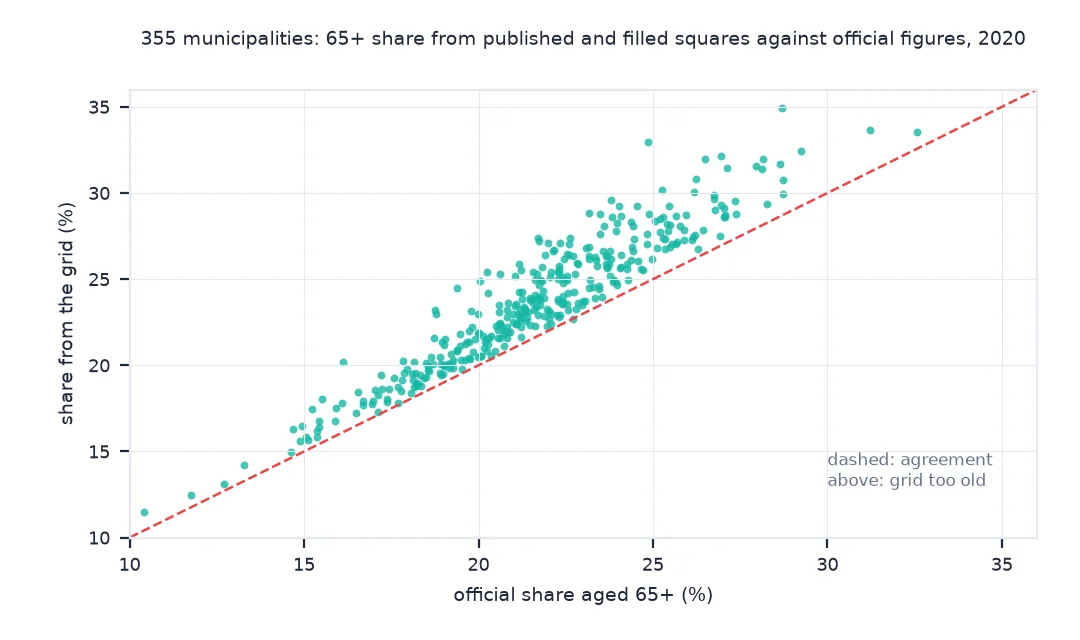
Sum each municipality's squares, published and filled, and compare the 65+ share with the official one:

pts = gpd.GeoDataFrame({"total": pub.aantal_inwoners, "old": filled.aantal_inwoners_65_jaar_en_ouder,
                        "known": filled.aantal_inwoners_65_jaar_en_ouder.notna()},
                       geometry=gpd.points_from_xy(pub.x * 100 + 50, pub.y * 100 + 50), crs=28992).sjoin(GM[["statcode", "geometry"]])
M = pts.groupby("statcode").apply(lambda g: g.old.sum() / g.total[g.known].sum(), include_groups=False).rename("grid").to_frame()
M["official"] = (AGE.k_65Tot80Jaar_8 + AGE.k_80JaarOfOuder_9) / AGE.TotaleBevolking_1
d = M.grid - M.official
print(f"{len(M)} municipalities: correlation {M.grid.corr(M.official):.3f}; median difference {d.median() * 100:+.1f} points; "
      f"within 1 point: {(d.abs() <= 0.01).mean():.0%}")
print(f"oldest by the grid: {GM.set_index('statcode').statnaam[M.grid.idxmax()]} {M.grid.max():.0%} (official {M.official[M.grid.idxmax()]:.0%})")

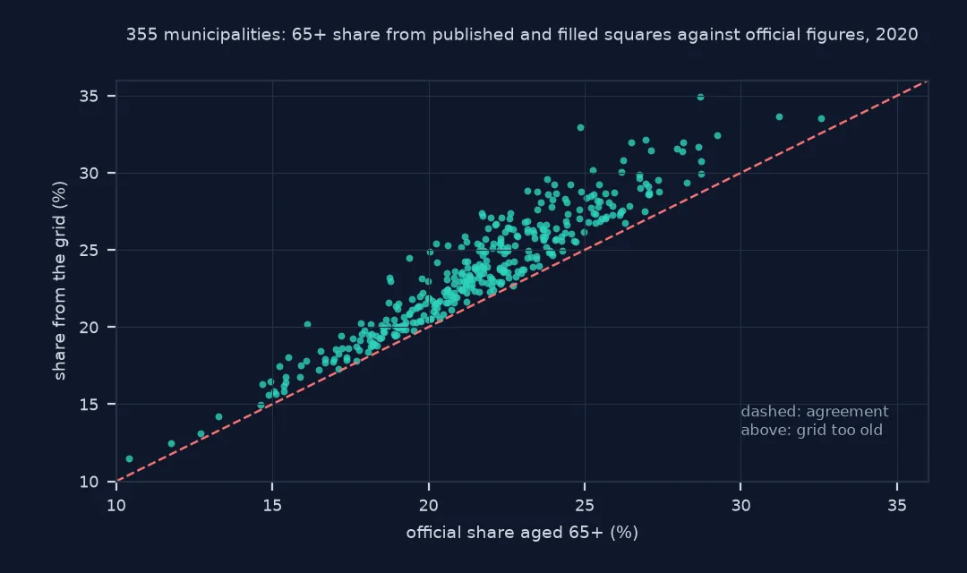
355 municipalities: correlation 0.948; median difference +1.6 points; within 1 point: 24%
oldest by the grid: Westerveld 35% (official 29%)

Aggregated to municipalities, the grid's 65+ shares track the official ones closely, with a correlation of 0.948, but they are too high by a median of 1.6 percentage points, and only a quarter are within one point. The grid's oldest municipality, Westerveld, comes out at 35% against an official 29%: the suppression bias from the quick answer, surviving aggregation.

Suppression is not random

Suppression in a census grid is not random. A band is suppressed where its count would be small enough to identify people, which happens in thinly populated squares and in squares dominated by one group. A share computed only from squares where the band survived therefore over-represents squares where the band is large. That is why the share of over-65s from published squares alone differs from the official one.

Recovering a band from the total works because the bands are a partition: they add up to the residents of the square, up to rounding. With exactly one band missing, the residual is the band, give or take the rounding of the other four; with two or more missing, the residual only bounds their sum. Aggregating to 1 km before computing shares adds back the residents of many squares and keeps the share defined, at the cost of resolution, and comparing with official municipal figures shows how far the result can be trusted.

Rounding, coverage and modelled grids

• Rounding adds up: each published count is rounded down to a multiple of five, so a residual can be off by up to 20 people in either direction; clip negative residuals to zero.
• Coverage threshold: the 80% coverage rule for 1 km cells is a choice; report it, and show cells below it as missing rather than as zero.
• Other attributes: households, dwellings by age and migration background are suppressed in the same way; the same partition trick works wherever categories add up to a published total.
• Modelled age grids: some global products estimate age structure per cell by disaggregating national or regional pyramids; they are smooth by construction and say little about where an age group concentrates within a municipality.

Internal links

• How to use a census population grid in Python — reading the grid and its codes
• Fixing a census grid total that comes out below the official population — the shortfall in totals
• How to suppress small counts in Python — the rules from the publisher's side

FAQ

How do I map the share of older people from a census grid?

Mask the suppression code, fill single suppressed bands from the square total where possible, aggregate to cells or areas large enough that most residents are covered, and divide the band by the total of the squares where it is known.

Why does my age share differ from the official figure?

Bands are suppressed where they are small, so a share from published squares only is biased; compare with official area totals and report the coverage.

Can suppressed values be recovered?

Only partly: where one category of a partition is suppressed, total minus the others recovers it to within the rounding; with two or more missing it cannot be separated.

Which age groups does the CBS grid have?

Under 15, 15 to 25, 25 to 45, 45 to 65, and 65 and over.