How to Detect Ocean Temperature Fronts in Python

Problem statement

An ocean front is a narrow zone where water temperature changes quickly over distance, the edge of a current or the boundary between water masses. Fronts concentrate plankton and fish, steer storms, and mark currents such as the Gulf Stream, whose northern edge, the "north wall", can change by 10 °C within tens of kilometres. Finding them in a sea surface temperature grid means computing the horizontal gradient correctly in kilometres, not degrees, and then deciding how strong a gradient counts as a front.

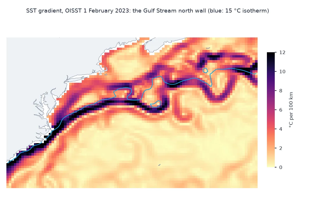
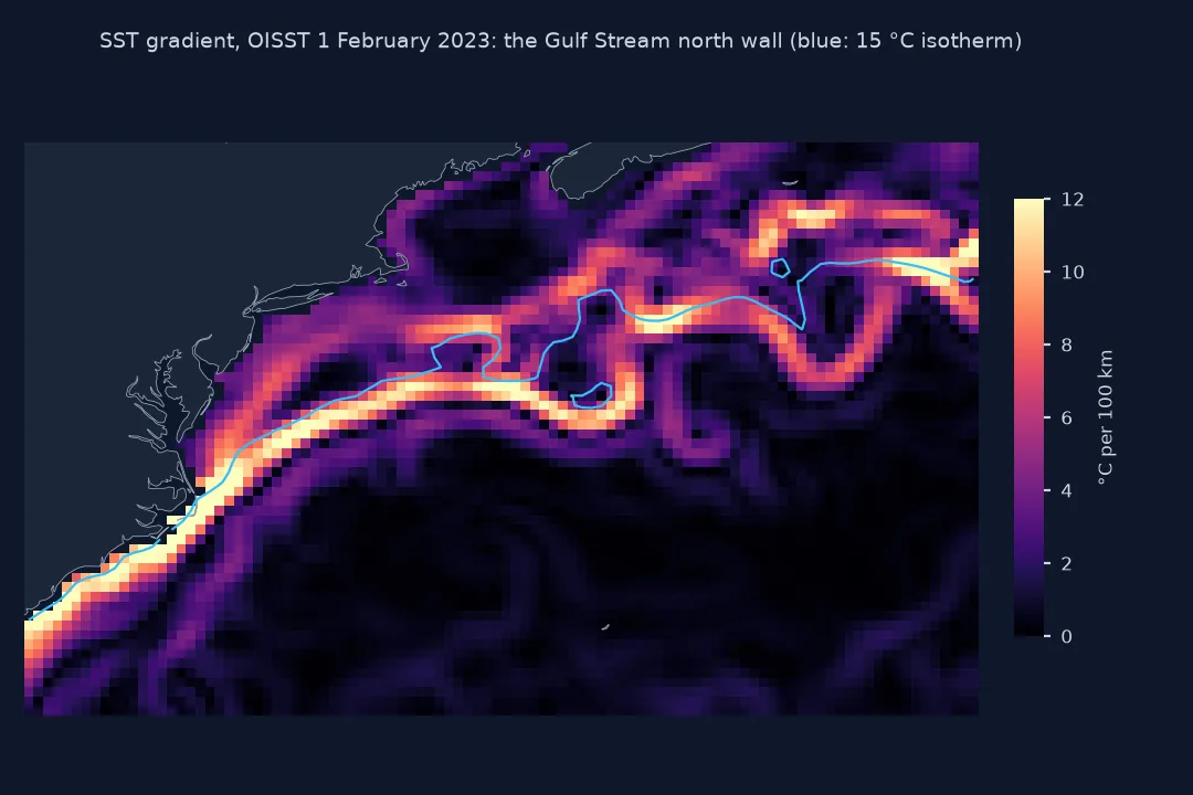
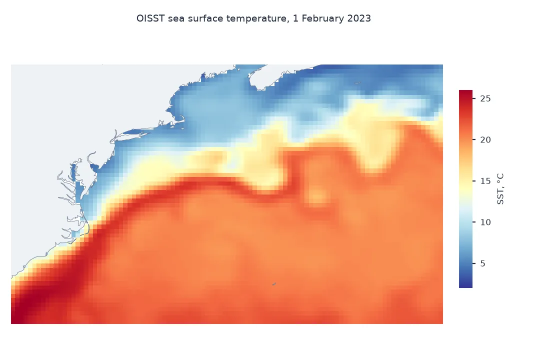
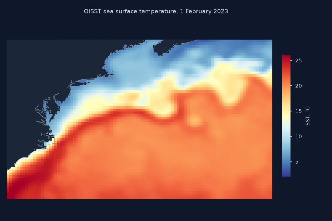
This page computes the temperature gradient of NOAA OISST off the US east coast on 1 February 2023, maps its strength, locates the Gulf Stream's north wall along several meridians, and checks how sensitive the result is to the threshold.

Quick answer

Convert the grid spacing to kilometres, take the gradient with NumPy, and report it per 100 km:

dy = 0.25 * 111.32                                                       # km per cell north-south
dx = 0.25 * 111.32 * np.cos(np.deg2rad(T.latitude.values))[:, None]      # km per cell east-west, by row
gy, gx = np.gradient(T.values)
G = np.hypot(gx / dx, gy / dy) * 100                                      # °C per 100 km
print(f"cells: {np.isfinite(G).sum():,}; median gradient {np.nanmedian(G):.2f} °C per 100 km; strongest {np.nanmax(G):.1f}")
print(f"cells above 5 °C per 100 km: {int(np.nansum(G > 5)):,} ({np.nanmean(G > 5):.1%})")

cells: 4,717; median gradient 1.01 °C per 100 km; strongest 18.8
cells above 5 °C per 100 km: 663 (11.1%)

Across 4,717 ocean cells the median gradient on 1 February 2023 is 1.01 °C per 100 km, and the strongest 18.8 °C per 100 km. 663 cells, 11.1%, exceed 5 °C per 100 km.

Degrees are the wrong unit, the north wall, threshold choice

1. Why degrees are the wrong unit

A gradient per degree of longitude is larger, for the same temperature change, the further north it is measured, because a degree of longitude shrinks. Compare the two at the box's edges:

for lat in (30, 45):
    print(f"{lat} N: one 0.25° cell is {0.25 * 111.32 * np.cos(np.radians(lat)):.1f} km east-west and {0.25 * 111.32:.1f} km north-south")
naive = np.hypot(gx, gy) / 0.25                                           # °C per degree, ignoring the shrinking longitude
print(f"correlation of per-degree and per-km gradient: {np.corrcoef(naive[np.isfinite(G)], G[np.isfinite(G)])[0, 1]:.3f}")

30 N: one 0.25° cell is 24.1 km east-west and 27.8 km north-south
45 N: one 0.25° cell is 19.7 km east-west and 27.8 km north-south
correlation of per-degree and per-km gradient: 0.996

Within this box a cell's east-west size shrinks from 24.1 km at 30°N to 19.7 km at 45°N. The per-degree and per-kilometre gradients still correlate at 0.996 here, so the pattern looks similar, but the values are not comparable, and over a larger range of latitude the difference grows.

2. The north wall along meridians

Along each meridian, the north wall is where the temperature drops fastest going north, south of the continental shelf. Find the latitude of the strongest gradient between 33°N and 43°N:

for lon in (-75, -72, -69, -66, -63, -60):
    col = T.sel(longitude=lon, method="nearest").sel(latitude=slice(33, 43))
    g = -np.gradient(col.values) / dy * 100
    i = int(np.nanargmax(g))
    print(f"{abs(lon)} W: strongest drop {g[i]:.1f} °C per 100 km at {float(col.latitude[i]):.2f} N, from {col.values[max(i - 2, 0)]:.1f} to {col.values[min(i + 2, len(col) - 1)]:.1f} °C")

75 W: strongest drop 13.2 °C per 100 km at 35.88 N, from 23.7 to 12.3 °C
72 W: strongest drop 10.6 °C per 100 km at 37.88 N, from 23.2 to 14.3 °C
69 W: strongest drop 9.5 °C per 100 km at 38.62 N, from 22.7 to 15.4 °C
66 W: strongest drop 9.3 °C per 100 km at 37.88 N, from 22.1 to 15.0 °C
63 W: strongest drop 11.0 °C per 100 km at 40.38 N, from 21.1 to 11.4 °C
60 W: strongest drop 4.9 °C per 100 km at 42.88 N, from 14.4 to 12.9 °C

Along most meridians the temperature falls by 9 to 13 °C per 100 km at the north wall, dropping as much as 11 °C across it: at 75°W from 23.7 to 12.3 °C near 35.9°N, at 69°W near 38.6°N. The wall's latitude meanders, back to 37.9°N at 66°W and up to 40.4°N at 63°W, and by 60°W the front has weakened to 4.9 °C per 100 km.

3. How much the threshold matters

There is no universal value for "a front". Count the frontal cells for several thresholds:

for thr in (2, 3, 5, 8):
    print(f"threshold {thr} °C per 100 km: {np.nanmean(G > thr):.1%} of ocean cells")

threshold 2 °C per 100 km: 27.2% of ocean cells
threshold 3 °C per 100 km: 20.8% of ocean cells
threshold 5 °C per 100 km: 11.1% of ocean cells
threshold 8 °C per 100 km: 5.0% of ocean cells

The frontal area depends heavily on the threshold: 28% of the box at 2 °C per 100 km, 11% at 5, 5% at 8.

The Gulf Stream front as a line

The data used on this page

Daily NOAA OISST v2.1 for 1 February 2023, 30°N to 45°N and 80°W to 55°W, from NCEI's daily archive: NOAA CoastWatch's ERDDAP aggregation is missing this day, and asked for it, returns a neighbouring one, so the setup checks the date and fills it from the archive file.

import io
import time
from pathlib import Path

import numpy as np
import pandas as pd
import requests
import xarray as xr

Path("data").mkdir(exist_ok=True)
CW = "https://coastwatch.pfeg.noaa.gov/erddap/griddap"
ARCHIVE = "https://www.ncei.noaa.gov/data/sea-surface-temperature-optimum-interpolation/v2.1/access/avhrr"
def _get(url):
    for attempt in range(5):                                            # a busy ERDDAP answers 500 or 503
        r = requests.get(url, timeout=900)
        if r.status_code < 500:
            break
        time.sleep(30 * (attempt + 1))
    r.raise_for_status()
    return r
def _lon180(da):
    return da.assign_coords(longitude=(da.longitude + 180) % 360 - 180).sortby("longitude")
def oisst(start, end, path, var="sst", lat=(52, 54), lon=(-12, -10), step=1):
    """Daily OISST v2.1 for a box and dates, saved to path, longitudes -180 to 180. CoastWatch's ERDDAP
    aggregation (version 2 before 2016, the same analysis as v2.1 for those years), with every day it
    lacks taken from NCEI's daily archive: the aggregations skip days, and a skipped day is silent."""
    path = Path(path)
    if not path.exists():
        days = pd.date_range(start, end)
        ds = "ncdcOisst2Agg" if days[-1].year <= 2015 else "ncdcOisst21Agg"
        a, b = lon[0] % 360, lon[1] % 360
        got = []
        for lo in [(a, b)] if a <= b else [(a, 359.875), (0.125, b)]:          # across 0°, two requests
            q = (f"{var}[({start}T12:00:00Z):1:({end}T12:00:00Z)][(0.0)]"
                 f"[({lat[0]}):{step}:({lat[1]})][({lo[0]}):{step}:({lo[1]})]")
            got.append(xr.open_dataset(io.BytesIO(_get(f"{CW}/{ds}.nc?{q}").content))[var].load())
        da = _lon180(xr.concat(got, "longitude").squeeze("zlev", drop=True))
        da = da.sel(time=slice(start, f"{end}T23:59"))                       # a missing end day snaps past it
        for day in days.difference(pd.DatetimeIndex(da.time.values).normalize()):
            url = f"{ARCHIVE}/{day:%Y%m}/oisst-avhrr-v02r01.{day:%Y%m%d}.nc"
            d = xr.open_dataset(io.BytesIO(_get(url).content))[var].squeeze("zlev", drop=True)
            d = _lon180(d.rename(lat="latitude", lon="longitude"))
            d = d.sel(latitude=da.latitude, longitude=da.longitude, method="nearest")
            da = xr.concat([da, d.assign_coords(latitude=da.latitude, longitude=da.longitude).load()], "time")
        da.sortby("time").to_dataset(name=var).to_netcdf(path)
    return xr.open_dataset(path)[var]
T = oisst("2023-02-01", "2023-02-01", "data/oisst_gulfstream_20230201.nc", "sst", (30.125, 44.875), (-79.875, -55.125)).squeeze(drop=True)
print(f"{T.sizes['latitude']} x {T.sizes['longitude']} cells; {float(T.min()):.1f} to {float(T.max()):.1f} °C")

60 x 100 cells; 1.3 to 26.4 °C

The box is 60 by 100 cells, with temperatures from 1.3 to 26.4 °C.

Example 1: the front as a line

Trace a single contour, the 15 °C isotherm, which in winter lies close to the north wall, and compare its latitude with the strongest gradient along the same meridians:

import matplotlib
matplotlib.use("Agg")
import matplotlib.pyplot as plt
cs = plt.contour(T.longitude, T.latitude, T.values, levels=[15])
paths = [p for p in cs.get_paths() if len(p.vertices) > 50]
v = max(paths, key=lambda p: len(p.vertices)).vertices
plt.close()
for lon in (-72, -66, -60):
    near = v[np.argmin(np.abs(v[:, 0] - lon))]
    print(f"15 °C isotherm near {abs(lon)} W: {near[1]:.2f} N")
print(f"length of the main 15 °C contour: {len(v)} vertices")

15 °C isotherm near 72 W: 38.12 N
15 °C isotherm near 66 W: 39.82 N
15 °C isotherm near 60 W: 40.38 N
length of the main 15 °C contour: 202 vertices

The 15 °C isotherm follows the same front, at 38.1°N near 72°W, but its latitude rises eastwards, to 40.4°N at 60°W, while the strongest gradient meanders: an isotherm and a gradient maximum describe slightly different things.

Gradients in kilometres, not degrees

The horizontal temperature gradient is the rate of change of temperature with distance, combining the east-west and north-south rates into a magnitude. On a latitude-longitude grid the east-west spacing shrinks with the cosine of latitude, so the derivative must be divided by each row's spacing in kilometres; otherwise the same front looks stronger in the north. numpy.gradient uses central differences, which are smooth but treat the edge of a missing land cell as the edge of the array, so gradients next to the coast are less reliable.

Gradient thresholds and isotherms are two ways of turning a field into fronts. A threshold marks every steep zone, including small eddies and shelf fronts; an isotherm follows one water mass boundary but depends on the season, because the whole field warms and cools. More elaborate methods, such as the Cayula-Cornillon histogram algorithm used for operational front maps, look for bimodal temperature distributions in windows. On a 0.25° analysis, any method finds the broad structure of the Gulf Stream; sharper fronts need higher-resolution data such as MUR or single-pass satellite images.

Analysis smoothing, gaps and seasonality

• Analysis smoothing: OISST's interpolation smooths fronts, so its gradients are weaker than those in 1 km satellite data.
• Clouds and gaps: an analysis has no gaps; single-pass satellite data have cloud gaps that produce false gradients at their edges.
• Seasonality: the north wall is sharpest in winter, when cold shelf water meets the current; summer gradients are weaker.
• Direction: the gradient vector also gives the front's orientation, arctan2(gy, gx), useful for following a front along its length.

Internal links

• How to download NOAA OISST sea surface temperature in Python — the data
• How to map sea surface temperature anomalies in Python — the other common derived map
• Sea surface temperature explained — resolution and what analyses smooth

FAQ

How do I calculate an SST gradient in Python?

Use numpy.gradient on the temperature array and divide each component by the grid spacing in kilometres, which for longitude shrinks with the cosine of latitude; combine them with numpy.hypot.

What gradient counts as an ocean front?

There is no single value; thresholds of a few °C per 100 km are common for 0.25° data, and step 3 shows how the area changes with the choice.

Where is the Gulf Stream north wall?

On 1 February 2023, the latitudes of the strongest temperature drop along several meridians are printed in step 2.

Why are my gradients stronger in the north?

The gradient was probably computed per degree; a degree of longitude covers fewer kilometres at higher latitude, so convert to distance first.