How to Animate Transit Vehicles from a GTFS Schedule in Python

Problem statement

A GTFS feed is a timetable: which trips run on which days, and when each trip reaches each stop. It does not say where a vehicle is between stops. To animate a network — every train on the map, minute by minute — you have to put each vehicle somewhere along its route at each moment. That means picking the services that run on one date, reading clock times that can pass 24:00, interpolating between stops, and following the route's shape instead of cutting corners. The result is the schedule as a moving picture, and a count of vehicles in service at every minute of the day.

This page animates the morning of a weekday on BART, the San Francisco Bay Area's rapid transit system, from its published GTFS feed.

Quick answer

Turn stop_times into segments (travelling from one stop to the next, or standing at a platform), find the segment each train is in at each moment, and interpolate along the route shape:

def positions(t):
    """Every train in service at time t (a Timedelta since midnight) as points in EPSG:26910."""
    live = seg[(seg.t0 <= t) & (seg.t1 > t)]
    frac = ((t - live.t0) / (live.t1 - live.t0)).to_numpy()
    d = live.d0.to_numpy() + frac * (live.d1 - live.d0).to_numpy()
    pts = [SHAPES[s].interpolate(x) for s, x in zip(live.shape_id, d)]
    return gpd.GeoDataFrame({"route": live.route_id.to_numpy()}, geometry=pts, crs=26910)

at8 = positions(pd.Timedelta("08:00:00"))
print(f"{len(at8)} trains in service at 08:00 on {DAY:%a %d %b %Y}")

56 trains in service at 08:00 on Wed 16 Sep 2026

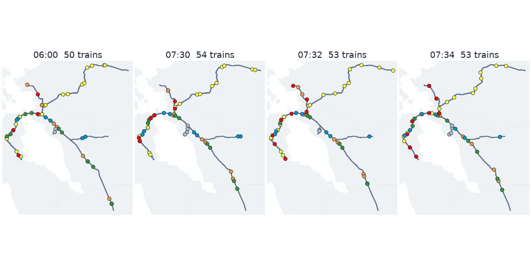
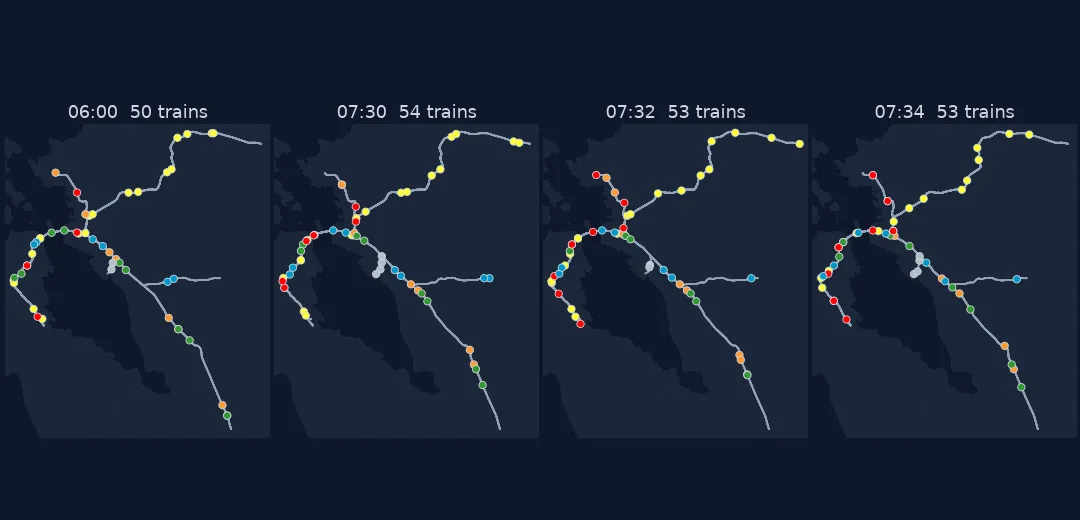
Services on the date, times as durations, distances along shapes

1. Pick the services that run on the date

calendar.txt gives weekly patterns with start and end dates; calendar_dates.txt adds or removes single days. Apply both:

cal = read("calendar")
dow = DAY.strftime("%A").lower()
on = set(cal.loc[(cal[dow] == "1") & (cal.start_date <= DAY) & (cal.end_date >= DAY), "service_id"])
ex = read("calendar_dates").query("date == @DAY")
on = (on | set(ex.loc[ex.exception_type == "1", "service_id"])) - set(ex.loc[ex.exception_type == "2", "service_id"])
day_trips = trips[trips.service_id.isin(on)]
print(f"feed version {info.feed_version.iloc[0]}: {len(on)} services and {len(day_trips):,} of {len(trips):,} trips run on {DAY:%a %d %b %Y}")

feed version 72: 3 services and 1,021 of 4,417 trips run on Wed 16 Sep 2026

2. Read times as durations, not clock times

A trip that starts at 23:50 and ends after midnight is written 24:20:00, still on the service day it started. Parse times as offsets from midnight, never as times of day:

late = st[st.arrival_time.str.slice(0, 2).astype(int) >= 24]
print(f"{len(late):,} stop times after midnight, latest {late.arrival_time.max()}")
print("pd.to_timedelta('24:20:00') =", pd.to_timedelta("24:20:00"))

1,996 stop times after midnight, latest 26:23:00
pd.to_timedelta('24:20:00') = 1 days 00:20:00

3. Measure each stop along its shape

To follow the track, each stop needs a distance along its trip's shape. shape_dist_traveled is optional and this feed leaves it empty, so project the stops onto the line. Projecting onto the whole shape goes wrong where a route doubles back: the Yellow line runs past Millbrae to SFO, reverses, and returns to Millbrae, so Millbrae lies on its shape twice. The setup's along() projects each stop only onto the part of the shape after the previous stop. Compare:

naive = pd.Series([SHAPES[k].project(shapely.Point(xy)) for k, xy in zip(s.shape_id, s.xy)], index=s.index)
print("shape_dist_traveled filled:", st.shape_dist_traveled.notna().sum())
print(f"whole-shape projection: {(naive.groupby(s.trip_id).diff() < 0).sum()} stop-to-stop moves run backwards; "
      f"forward-only projection: {(seg.d1 < seg.d0).sum()} of {len(seg):,} segments")

shape_dist_traveled filled: 0
whole-shape projection: 4 stop-to-stop moves run backwards; forward-only projection: 0 of 19,463 segments

A backwards move puts a train into reverse for a few minutes in the animation. Out-and-back and loop routes are where to look for them.

4. Follow the shape, not a straight line

Interpolating straight between stations is simpler, but it cuts every curve. Compare the two at one moment:

live = seg[(seg.t0 <= T) & (seg.t1 > T)]
frac = ((T - live.t0) / (live.t1 - live.t0)).to_numpy()
on_shape = [SHAPES[s].interpolate(a + f * (b - a)) for s, a, b, f in zip(live.shape_id, live.d0, live.d1, frac)]
straight = [shapely.Point(np.array(p0) + f * (np.array(p1) - np.array(p0))) for p0, p1, f in zip(live.xy0, live.xy1, frac)]
off = np.array([a.distance(b) for a, b in zip(on_shape, straight)])
print(f"at {str(T)[-8:-3]}: {len(off)} trains, straight-line position off the track by median {np.median(off):.0f} m, max {off.max():.0f} m")

at 08:00: 56 trains, straight-line position off the track by median 60 m, max 1299 m

5. Count vehicles in service through the day

The same segments give the number of trains in service at every minute, which is the animation's own summary:

minutes = pd.timedelta_range("04:00:00", "25:00:00", freq="1min")
counts = pd.Series([((seg.t0 <= m) & (seg.t1 > m)).sum() for m in minutes], index=minutes)
peak = counts.idxmax()
print(f"most trains in service: {counts.max()} at {str(peak)[-8:-3]}; at 08:00 {counts[pd.Timedelta('08:00:00')]}, "
      f"at 17:30 {counts[pd.Timedelta('17:30:00')]}, at 12:00 {counts[pd.Timedelta('12:00:00')]}; last arrival {str(seg.t1.max())}")
print(f"stop times with a dwell (departure after arrival): {(s.t_dep > s.t_arr).sum():,}")

most trains in service: 56 at 07:11; at 08:00 56, at 17:30 54, at 12:00 56; last arrival 1 days 01:52:00
stop times with a dwell (departure after arrival): 5,465

Dwell times are segments too, with the same distance at both ends, so a train standing at a platform is counted and drawn where it stands. Leave them out and every train with a dwell vanishes from the map while it waits.

BART's morning, animated

The data used on this page

The BART GTFS feed, feed version 72 (published August 2026; feed versions change, so the counts below belong to that version). Positions are computed in UTM zone 10N (EPSG:26910).

import io
import zipfile
from pathlib import Path

import geopandas as gpd
import imageio.v3 as iio
import matplotlib
matplotlib.use("Agg")
import matplotlib.pyplot as plt
import numpy as np
import pandas as pd
import requests
import shapely
import shapely.ops

Path("data").mkdir(exist_ok=True)
FEED = Path("data/bart_gtfs.zip")
if not FEED.exists():
    FEED.write_bytes(requests.get("https://www.bart.gov/dev/schedules/google_transit.zip", timeout=120).content)
Z = zipfile.ZipFile(FEED)
read = lambda name: pd.read_csv(Z.open(f"{name}.txt"), dtype=str).apply(
    lambda c: pd.to_datetime(c, format="%Y%m%d") if c.name in ("start_date", "end_date", "date") else c)
info, trips, st, stops, routes = read("feed_info"), read("trips"), read("stop_times"), read("stops"), read("routes")
cal = read("calendar")
for d in ("monday", "tuesday", "wednesday", "thursday", "friday", "saturday", "sunday"):
    cal[d] = cal[d].astype(int)
DAY = pd.Timestamp("2026-09-16")                                   # a Wednesday inside the feed's calendar

shp = read("shapes").astype({"shape_pt_lat": float, "shape_pt_lon": float, "shape_pt_sequence": int}).sort_values(["shape_id", "shape_pt_sequence"])
pts = gpd.GeoSeries(gpd.points_from_xy(shp.shape_pt_lon, shp.shape_pt_lat), crs=4326).to_crs(26910)
shp["x"], shp["y"] = pts.x.to_numpy(), pts.y.to_numpy()
SHAPES = {k: shapely.LineString(g[["x", "y"]].to_numpy()) for k, g in shp.groupby("shape_id")}
sxy = gpd.GeoSeries(gpd.points_from_xy(stops.stop_lon.astype(float), stops.stop_lat.astype(float)), crs=4326).to_crs(26910)
STOP_XY = dict(zip(stops.stop_id, zip(sxy.x, sxy.y)))

cal_on = set(cal.loc[(cal[DAY.strftime("%A").lower()] == 1) & (cal.start_date <= DAY) & (cal.end_date >= DAY), "service_id"])
exd = read("calendar_dates").query("date == @DAY")
cal_on = (cal_on | set(exd.loc[exd.exception_type == "1", "service_id"])) - set(exd.loc[exd.exception_type == "2", "service_id"])
s = st.merge(trips[trips.service_id.isin(cal_on)][["trip_id", "route_id", "shape_id"]], on="trip_id")
s["seq"] = s.stop_sequence.astype(int)
s = s.sort_values(["trip_id", "seq"])
s["t_arr"], s["t_dep"] = pd.to_timedelta(s.arrival_time), pd.to_timedelta(s.departure_time)
s["xy"] = s.stop_id.map(STOP_XY)


def along(g):
    """Distance of each stop along the shape, never behind the previous stop (shapes can double back)."""
    line, prev, out = SHAPES[g.shape_id.iloc[0]], 0.0, []
    for xy in g.xy:
        rest = shapely.ops.substring(line, prev, line.length)
        if rest.geom_type == "LineString":                         # a Point once prev reaches the end of the line
            prev += rest.project(shapely.Point(xy))
        out.append(prev)
    return pd.Series(out, index=g.index)


s["d"] = s.groupby("trip_id", group_keys=False)[["shape_id", "xy"]].apply(along)
ev = pd.concat([s.assign(t=s.t_arr, k=0), s.assign(t=s.t_dep, k=1)]).sort_values(["trip_id", "seq", "k"])
nxt = ev.groupby("trip_id").shift(-1)                              # arrive -> depart is a dwell, depart -> arrive a run
seg = pd.DataFrame({"trip_id": ev.trip_id, "route_id": ev.route_id, "shape_id": ev.shape_id, "t0": ev.t, "t1": nxt.t,
                    "d0": ev.d, "d1": nxt.d, "xy0": ev.xy, "xy1": nxt.xy}).dropna(subset=["t1"])
seg = seg[seg.t1 > seg.t0]
T = pd.Timedelta("08:00:00")
print(f"{len(SHAPES)} shapes, {len(stops)} stops, {len(seg):,} segments on {DAY:%d %b %Y}")

28 shapes, 287 stops, 19,463 segments on 16 Sep 2026

The setup's cal_on repeats step 1's selection so that the segments exist before the quick answer runs.

Example 1: render the morning

colour = dict(zip(routes.route_id, "#" + routes.route_color))
track = gpd.GeoSeries(list(SHAPES.values()), crs=26910)
x0, y0, x1, y1 = track.total_bounds
frames = []
for t in pd.timedelta_range("07:00:00", "09:00:00", freq="2min"):
    p = positions(t)
    fig, ax = plt.subplots(figsize=(5, 6), dpi=80)
    track.plot(ax=ax, color="#cccccc", lw=1)
    p.plot(ax=ax, color=[colour[r] for r in p.route], markersize=18, edgecolor="#333333", linewidth=0.4)
    ax.set_xlim(x0 - 2000, x1 + 2000); ax.set_ylim(y0 - 2000, y1 + 2000); ax.set_axis_off()
    ax.set_title(f"BART  {str(t)[-8:-3]}  {len(p)} trains", fontsize=10)
    fig.canvas.draw(); frames.append(np.asarray(fig.canvas.buffer_rgba())[..., :3].copy()); plt.close(fig)
iio.imwrite("data/bart_peak.gif", frames, duration=120, loop=0)
print(f"{len(frames)} frames, {Path('data/bart_peak.gif').stat().st_size / 1e6:.2f} MB")

61 frames, 0.28 MB

A schedule is a list of promises

A GTFS schedule is a list of promises at stops. An animation needs positions at moments, so the work is filling the gaps. Between two stops the schedule says only "left here at t0, arrives there at t1". The simplest honest assumption is constant speed along the track for that interval. That is what interpolating along the shape does, and why the shape matters: straight lines between stations cut the curves and put trains off the track.

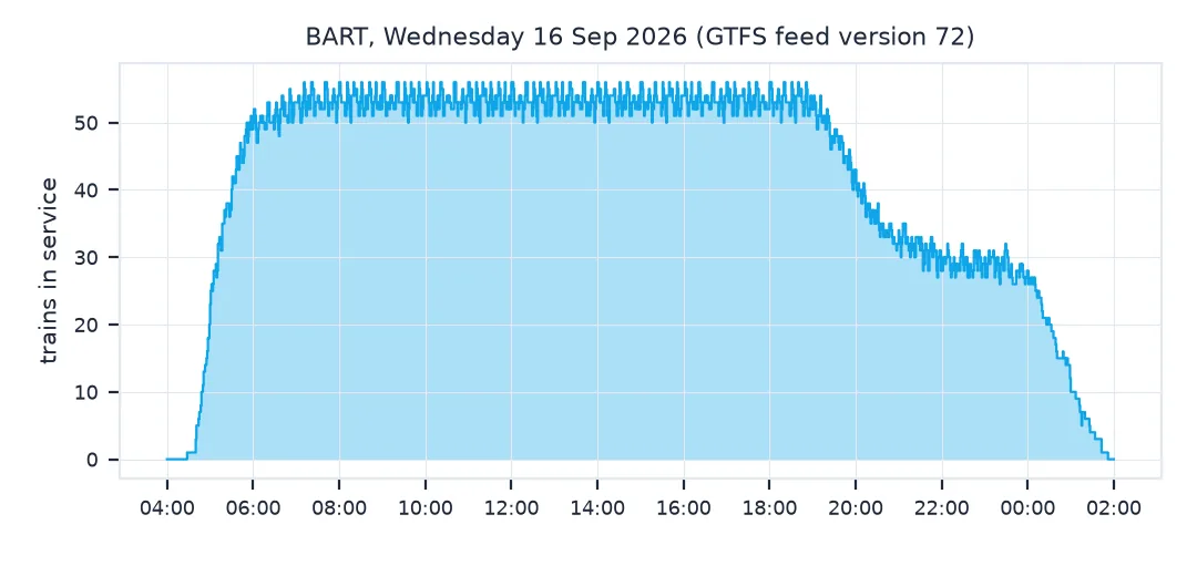
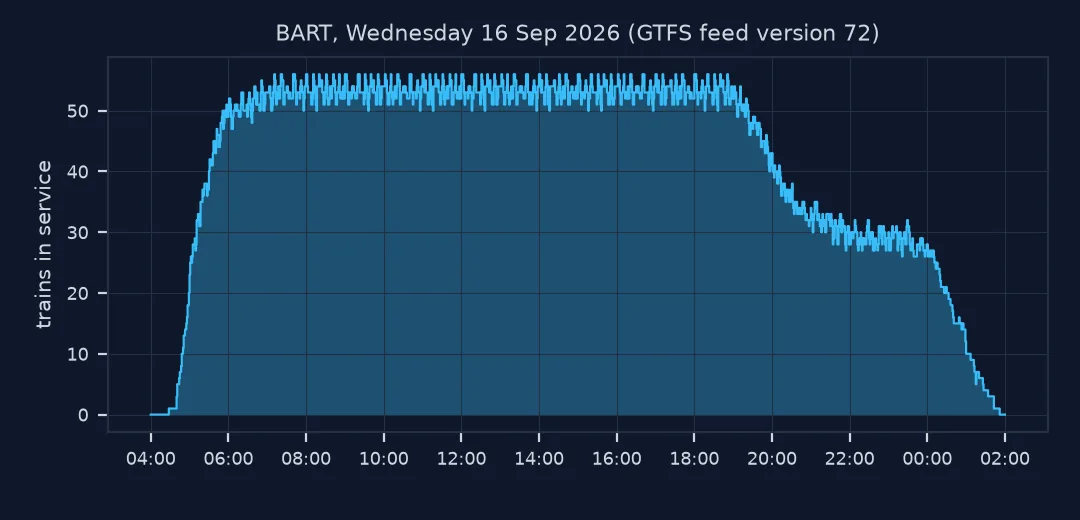
The service calendar and the clock are the two traps that make an animation wrong without looking wrong. Use the wrong services and the map fills with weekend trains on a Wednesday, or with trips from a timetable that has already ended. Parse times as clock times and every trip that runs past midnight vanishes or wraps to the morning. Both are checked above with counts. The vehicle count through the day is a quick sanity check against the published timetable. For BART in this feed it shows no commuter peaks at all: a flat 50 to 56 trains from 7 am to 7 pm, about 30 in the late evening, and the last arrival at 01:52.

Realtime positions, dwell times and loops

• Real-time positions come from GTFS-Realtime VehiclePositions, a different feed; this page animates the plan, not what happened.
• Frequency-based trips (frequencies.txt) list one template trip and a headway; expand them into individual trips first.
• Dwell times are part of the schedule; build a segment for each one, or trains disappear while they stand at platforms.
• Stops without times (timepoint = 0, blank times) need interpolating before segments can be built.
• Loops and out-and-back shapes make projection ambiguous; project each stop onto the part of the shape after the previous stop.
• Time zone comes from agency_timezone; times are local, including daylight saving.
• Feed versions change every few months; record the version you animated.

Internal links

• How to make an animated map — the frame loop and export
• How to make an earthquake sequence animation — events rather than vehicles

FAQ

How do I get vehicle positions from GTFS?

Schedule positions: build stop-to-stop and dwell segments from stop_times, find the one each trip is in at time t, and interpolate along the trip's shape. Live positions come from a GTFS-Realtime feed instead.

Why does GTFS have times like 25:30:00?

Times are measured from noon minus 12 hours on the service day, so trips after midnight keep counting past 24:00. Parse them with pd.to_timedelta.

How do I find which trips run on a given date?

Take the services whose weekday flag is set and whose date range covers the date in calendar.txt, add calendar_dates.txt additions (type 1), and remove its exceptions (type 2).

Why are my animated vehicles off the track?

They are being interpolated in a straight line between stops; interpolate distance along the trip's shape instead.