
How to Relate Daily Crime to Temperature in Python
On this page
Problem statement
Violent crime rises in warm weather, one of the oldest findings in criminology. Testing it on a city's own data looks like a scatter plot of daily counts against daily temperature, and the correlation that comes out is strong. Most of it, though, is the calendar: summer is warm, summer has long evenings, school holidays and more people outdoors, and anything with a summer peak will correlate with temperature. The question worth answering is whether a day that is warmer than usual for its time of year has more crime than a typical day of that month.
This page joins daily counts of eight offence types in Chicago from 2019 to 2024 to the daily maximum temperature at O'Hare from NOAA's GHCN-Daily, measures the raw correlation, removes the month and the day of the week, and estimates how many more incidents each extra degree brings.
Quick answer
Subtract each month's mean and each weekday's mean from the daily counts, take temperature as its difference from the month's mean, and correlate the two anomalies:
def anomaly(col):
    a = D[col] - D.groupby("month")[col].transform("mean")
    return a - a.groupby(D.index.dayofweek).transform("mean")

t_anom = D.tmax - D.groupby("month").tmax.transform("mean")
for col in ("BATTERY", "ASSAULT", "ROBBERY", "DECEPTIVE PRACTICE"):
    a = anomaly(col)
    slope = np.polyfit(t_anom, a, 1)[0]
    print(f"{col.lower():19s} raw r = {D[col].corr(D.tmax):+.2f}, within month r = {a.corr(t_anom):+.2f}, "
          f"{slope:+.2f} a day per °C ({slope / D[col].mean():+.1%})")
battery raw r = +0.50, within month r = +0.41, +1.27 a day per °C (+1.1%)
assault raw r = +0.56, within month r = +0.32, +0.53 a day per °C (+0.9%)
robbery raw r = +0.17, within month r = +0.11, +0.14 a day per °C (+0.6%)
deceptive practice raw r = -0.10, within month r = +0.02, +0.06 a day per °C (+0.1%)
Removing the month and the weekday lowers every correlation, assault's most, from 0.56 to 0.32. What survives is a steady effect: about 1.27 more batteries a day for each degree above the month's average, 1.1% of the daily mean. Deceptive practice, the control, has a raw correlation of -0.10 and a within-month one of 0.02.
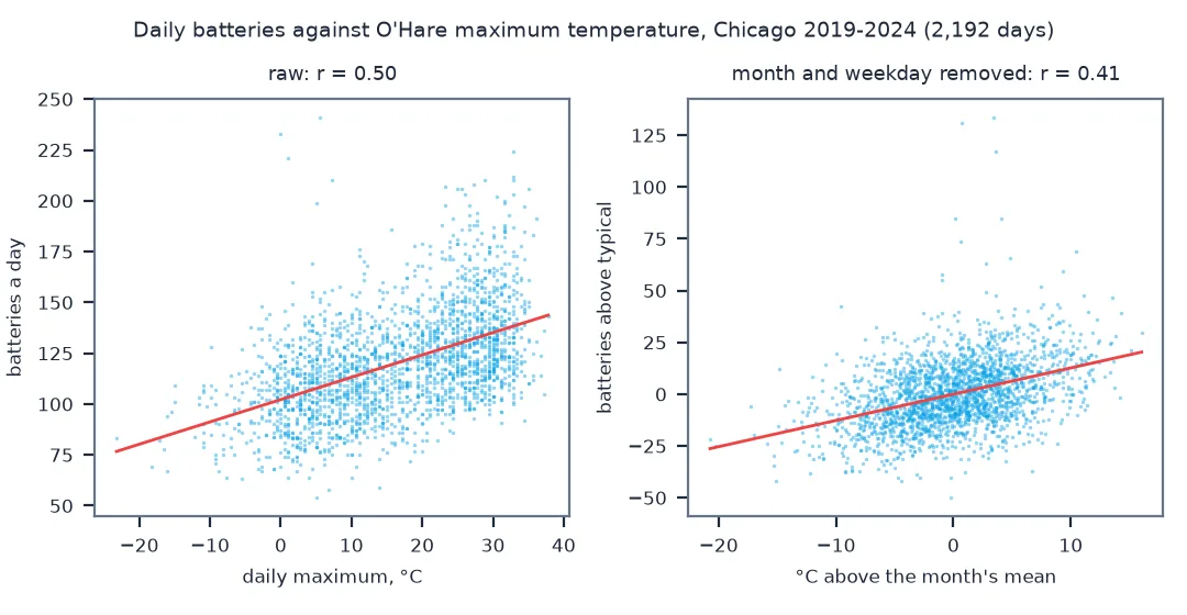
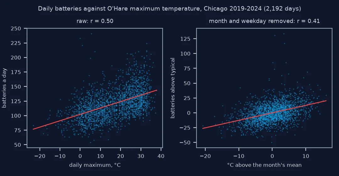
Join daily series, remove the season, look at the shape
1. Join the two daily series
Weather stations report by local standard day; crime counts are by calendar day in Chicago time. For daily totals the two line up closely enough; check that no day is missing:
print(f"{len(D):,} days, {D.index.min():%d %b %Y} to {D.index.max():%d %b %Y}; days without a temperature: {D.tmax.isna().sum()}")
print(f"daily maximum at O'Hare: {D.tmax.min():.1f} to {D.tmax.max():.1f} °C; mean batteries a day: {D.BATTERY.mean():.0f}")
2,192 days, 01 Jan 2019 to 31 Dec 2024; days without a temperature: 0
daily maximum at O'Hare: -23.2 to 37.8 °C; mean batteries a day: 120
All 2,192 days have a temperature, from -23.2 °C to 37.8 °C; the city recorded 120 batteries on an average day.
2. See how much is season
The month alone explains a large part of the daily variation in battery counts, as it does for temperature:
for col in ("BATTERY", "tmax"):
    share = D.groupby("month")[col].transform("mean").var() / D[col].var()
    print(f"{col}: month means explain {share:.0%} of the day-to-day variance")
print(f"calendar months, 2019-2024: {D.month.nunique()}")
BATTERY: month means explain 38% of the day-to-day variance
tmax: month means explain 79% of the day-to-day variance
calendar months, 2019-2024: 72
The 72 month means explain 79% of the variance in daily maximum temperature and 38% of the variance in daily batteries. Correlating the raw series lets that shared calendar carry much of the result.
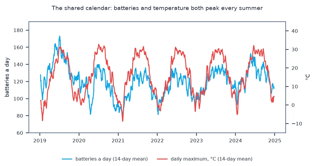
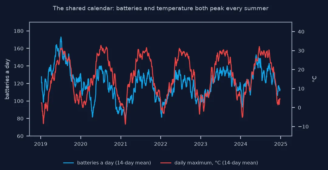
3. Look at the shape
A slope assumes a straight line. Average the battery anomaly in bands of temperature anomaly:
bands = pd.cut(t_anom, [-20, -8, -4, -1, 1, 4, 8, 20])
curve = anomaly("BATTERY").groupby(bands, observed=True).agg(["mean", "size"])
print(curve.round(1).to_string())
mean size
tmax
(-20, -8] -13.0 131
(-8, -4] -7.6 333
(-4, -1] -3.2 458
(-1, 1] 0.8 320
(1, 4] 3.3 479
(4, 8] 5.5 327
(8, 20] 14.7 142
The battery anomaly rises through every band, from 13 fewer a day on the coldest days for the month to 14.7 more on the warmest, and the step is largest at the warm end: from 5.5 to 14.7 between the last two bands.
Hot and cool days in the same month
The data used on this page
Daily counts by offence type from the City of Chicago's Crimes - 2001 to Present (ijzp-q8t2), aggregated on the server with SoQL for 2019–2024; and the daily maximum temperature (TMAX, tenths of a degree Celsius) at Chicago O'Hare International Airport, station USW00094846, from NOAA's GHCN-Daily.
from pathlib import Path

import numpy as np
import pandas as pd
import requests

Path("data").mkdir(exist_ok=True)
TYPES = ["BATTERY", "ROBBERY", "THEFT", "ASSAULT", "MOTOR VEHICLE THEFT", "BURGLARY", "HOMICIDE", "DECEPTIVE PRACTICE"]
F = Path("data/daily.json")
if not F.exists():
    F.write_bytes(requests.get("https://data.cityofchicago.org/resource/ijzp-q8t2.json", timeout=300, params={
        "$select": "date_trunc_ymd(date) AS day, primary_type, count(*) AS n",
        "$where": "year BETWEEN 2019 AND 2024 AND primary_type IN (" + ", ".join(f"'{t}'" for t in TYPES) + ")",
        "$group": "day, primary_type", "$limit": 50_000}).content)
W = Path("data/USW00094846.csv")
if not W.exists():
    W.write_bytes(requests.get("https://www.ncei.noaa.gov/data/global-historical-climatology-network-daily/access/USW00094846.csv", timeout=300).content)
d = pd.read_json(F).assign(day=lambda x: pd.to_datetime(x.day))
D = d.pivot_table(index="day", columns="primary_type", values="n", aggfunc="sum").reindex(columns=TYPES).fillna(0)
w = pd.read_csv(W, usecols=["DATE", "TMAX"], parse_dates=["DATE"]).set_index("DATE")
D["tmax"] = w.TMAX.reindex(D.index) / 10                               # tenths of °C to °C
D["month"] = D.index.to_period("M")
print(f"{len(D):,} days; {int(D[TYPES].values.sum()):,} incidents of {len(TYPES)} types")
2,192 days; 1,022,038 incidents of 8 types
Example 1: hot days and cool days in the same month
The plainest version of the test: within each month, compare the five warmest days with the five coolest:
rank = D.groupby("month").tmax.rank(method="first")
size = D.groupby("month").tmax.transform("size")
hot, cool = rank > size - 5, rank <= 5
for col in ("BATTERY", "ASSAULT", "HOMICIDE", "DECEPTIVE PRACTICE"):
    print(f"{col.lower():19s} warmest 5 days {D.loc[hot, col].mean():6.1f} a day, coolest 5 {D.loc[cool, col].mean():6.1f} "
          f"({D.loc[hot, col].mean() / D.loc[cool, col].mean() - 1:+.0%})")
print(f"temperature: warmest 5 average {D.loc[hot, 'tmax'].mean():.1f} °C, coolest 5 {D.loc[cool, 'tmax'].mean():.1f} °C")
battery warmest 5 days 128.5 a day, coolest 5 111.3 (+15%)
assault warmest 5 days 60.5 a day, coolest 5 53.6 (+13%)
homicide warmest 5 days 2.2 a day, coolest 5 1.6 (+42%)
deceptive practice warmest 5 days 49.3 a day, coolest 5 49.0 (+1%)
temperature: warmest 5 average 23.5 °C, coolest 5 8.7 °C
Within the same months, the five warmest days averaged 23.5 °C against 8.7 °C for the five coolest, and had 15% more batteries and 13% more assaults. Homicides were 42% more frequent, on averages of 2.2 and 1.6 a day; deceptive practice differed by 1%.
Season and temperature are mixed together
The raw correlation between daily crime and temperature mixes two things. One is the season: everything that changes between January and July, of which temperature is only one part. The other is the effect of weather itself: on a day warmer than usual for the time of year, more people are out, for longer, which raises the chances of confrontations and of street crime. Removing the month's mean from both series takes out the season, and what is left is the day-to-day relationship. Removing the weekday mean as well stops the weekend peak from blurring it.
The method is a simple version of the fixed-effects regressions used in the research literature, with month and weekday as the fixed effects. Its result is smaller than the raw correlation suggests, but not small: battery and assault rise by about one percent per degree on a day warmer than usual, while deceptive practice, mostly fraud reported after the fact, shows almost nothing, which is what a weather effect predicts and a calendar artefact would not.
Temperature is also a stand-in. Hot days are often dry and long, and rain keeps people indoors; precipitation, daylight and holidays are the next variables to add, and the lagged effect of a heatwave is a question of its own.
One station, counts and overdispersion
- One station for a city: O'Hare sits at the city's north-west edge; neighbourhood temperatures differ, especially near the lake, but the day-to-day variation is shared.
- Counts, not rates: daily counts assume a stable population over the period, which holds for a few years.
- 2020: lockdowns changed crime and mobility at once; month means absorb the level shift, and a sensitivity check without 2020 is worth running.
- Midnight records: incidents recorded at exactly 00:00 have uncertain dates as well as times; for daily counts the effect is small.
- Overdispersion: for a formal model, use a negative binomial regression with month and weekday terms, which gives standard errors as well as the slope.
Internal links
- How to analyse crime by hour and day of week in Python — the weekly and daily cycle
- How to analyse crime trends over time in Python — season and trend
- How to compare air temperature with land surface temperature in Python — temperature data
FAQ
Does hot weather increase crime?
In Chicago from 2019 to 2024, a day warmer than usual for its month had about 1% more batteries and assaults per degree Celsius; fraud showed no such effect.
How do I remove seasonality from daily crime data?
Subtract each month's mean, and each weekday's mean, from the daily counts, and use the temperature's difference from its monthly mean.
Where can I get daily temperature data for a city?
NOAA's GHCN-Daily has daily maximum and minimum temperature and precipitation for thousands of stations, one CSV per station.
Why is the raw correlation between crime and temperature misleading?
Because both follow the season; much of the correlation is summer against winter, which includes daylight, holidays and other changes as well as temperature.